Wavelet for Graphs and its Deployment to Image Processing
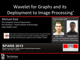
Wavelet for Graphs and its Deployment to Image Processing . Michael Elad The Computer Science Department The Technion – Israel Institute of technology Haifa 32000, Israel.

Wavelet for Graphs and its Deployment to Image Processing
E N D
Presentation Transcript
Wavelet for Graphs and its Deployment to Image Processing Michael Elad The Computer Science Department The Technion – Israel Institute of technology Haifa 32000, Israel The research leading to these results has been received funding from the European union's Seventh Framework Program (FP/2007-2013) ERC grant Agreement ERC-SPARSE- 320649
This Talk is About … Processing of Non-Conventionally Structured Signals As you will see, we will use the developed tools to process “regular” signals (e.g., images) , handling them differently and more effectively Many signal-processing tools (filters, alg., transforms, …) are tailored for uniformly sampled signals Now we encounter different types of signals: e.g., point-clouds and graphs. Can we extend classical tools to these signals? Our goal: Generalize the wavelet transform to handle this broad family of signals The true objective: Find how to bring sparse representation to processing of such signals 2
This is Joint Work With • I. Ram, M. Elad, and I. Cohen, “Generalized Tree-Based Wavelet Transform”, IEEE Trans. Signal Processing, vol. 59, no. 9, pp. 4199–4209, 2011. • I. Ram, M. Elad, and I. Cohen, “Redundant Wavelets on Graphs and High Dimensional Data Clouds”, IEEE Signal Processing Letters, Vol. 19, No. 5, pp. 291–294 , May 2012. • I. Ram, M. Elad, and I. Cohen, “The RTBWT Frame – Theory and Use for Images”, to appear in IEEE Trans. on Image Processing. • I. Ram, M. Elad, and I. Cohen, “Image Processing using Smooth Ordering of its Patches”, IEEE Transactions on Image Processing, Vol. 22, No. 7, pp. 2764–2774 , July 2013. • I. Ram, I. Cohen, and M. Elad, “Facial Image Compression using Patch-Ordering-Based Adaptive Wavelet Transform”, Submitted to IEEE Signal Processing Letters. Idan Ram Israel Cohen The EE department - the Technion 3
Part I – GTBWT Generalized Tree-Based Wavelet Transform – The Basics This part is taken from the following two papers : • I. Ram, M. Elad, and I. Cohen, “Generalized Tree-Based Wavelet Transform”, IEEE Trans. Signal Processing, vol. 59, no. 9, pp. 4199–4209, 2011. • I. Ram, M. Elad, and I. Cohen, “Redundant Wavelets on Graphs and High Dimensional Data Clouds”, IEEE Signal Processing Letters, Vol. 19, No. 5, pp. 291–294 , May 2012. 4
Problem Formulation • We are given a graph: • The node is characterized by a -dimen. feature vector • The node has a value • The edge between the and nodes carries the distance for an arbitrary distance measure . • Assumption: a “short edge” implies close-by values, i.e. smallsmall for almost every pair . 5
A Different Way to Look at this Data • We start with a set of -dimensional vectors These could be: • Feature points for a graph’s nodes, • Set of coordinates for a point-cloud. • A scalar function is defined on these coordinates, , giving . • We may regard this dataset as a set of samples taken from a high dimensional function . • The assumption that small implies small for almost every pair implies that the function behind the scene, , is “regular”. X= … … 6
Our Goal X Sparse (compact) Representation Wavelet Transform • Why Wavelet? • Wavelet for regular piece-wise smooth signals is a highly effective “sparsifying transform”. However, the signal (vector) f is not necessarily smooth in general. • We would like to imitate this for our data structure. 7
Wavelet for Graphs – A Wonderful Idea I wish we would have thought of it first … “Diffusion Wavelets” R. R. Coifman, and M. Maggioni, 2006. “Multiscale Methods for Data on Graphs and Irregular …. Situations” M. Jansen, G. P. Nason, and B. W. Silverman, 2008. “Wavelets on Graph via SpectalGraph Theory” D. K. Hammond, and P. Vandergheynst, and R. Gribonval, 2010. “Multiscale Wavelets on Trees, Graphs and High … Supervised Learning” M . Gavish, and B. Nadler, and R. R. Coifman, 2010. “Wavelet Shrinkage on Paths for Denoising of Scattered Data” D. Heinen and G. Plonka, 2012. … 8
The Main Idea (1) - Permutation Permutation using Permutation 1D Wavelet P T T-1 P-1 Processing 9
The Main Idea (2) - Permutation • In fact, we propose to perform a different permutation in each resolution level of the multi-scale pyramid: • Naturally, these permutations will be applied reversely in the inverse transform. • Thus, the difference between this and the plain 1D wavelet transform applied on f are the additional permutations, thus preserving the transform’s linearity and unitarity, while also adapting to the input signal. 10
Building the Permutations (1) • Lets start with P0 – the permutation applied on the incoming signal. • Recall: the wavelet transform is most effective for piecewise regular signals. → thus, P0 should be chosen such that P0f is most “regular”. • Lets use the feature vectors in X, reflecting the order of the values, fk. Recall: • Thus, instead of solving for the optimal permutation that “simplifies” f, we order the features in X to the shortest path that visits in each point once, in what will be an instance of the Traveling-Salesman-Problem (TSP): Small implies small for almost every pair 11
Building the Permutations (2) • We handle the TSP task by a greedy (and crude) approximation: • Initialize with an arbitrary index j; • Initialize the set of chosen indices to Ω(1)={j}; • Repeat k=1:1:N-1 times: • Find xi– the nearest neighbor to xΩ(k) such that iΩ; • Set Ω(k+1)={i}; • Result: the set Ωholds the proposed ordering. 12
Building the Permutations (3) • So far we concentrated on P0 at the finest level of the multi-scale pyramid. • In order to construct P1, P2, … ,PL-1, the permutations at the other pyramid’s levels, we use the same method, applied on propagated (reordered, filtered and sub-sampled) feature-vectors through the same wavelet pyramid: P1 P0 LP-Filtering (h) & Sub-sampling LP-Filtering (h) & Sub-sampling P3 LP-Filtering (h) & Sub-sampling P2 LP-Filtering (h) & Sub-sampling 13
Why “Generalized Tree …”? • “Generalized” tree Tree (Haar wavelet) • Our proposed transform: Generalized Tree-Based Wavelet Transform (GTBWT). • We also developed a Redundant version of this transform based on the stationary wavelet transform [Shensa, 1992][Beylkin, 1992]– also related to the “A-TrousWavelet” (will not be presented here). 14
Treating Graph/Cloud-of-points • Just to complete the picture, we should demonstrate the (R)GTBWT capabilities on graphs/cloud of points. • We took several classical machine learning train + test data for several regression problems, and tested the proposed transform in • Cleaning (denoising) the data from additive noise; • Filling in missing values (semi-supervised learning); and • Detecting anomalies (outliers) in the data. • The results are encouraging. We shall present herein one such experiment briefly. SKIP? 15
Treating Graphs: The Data Data Set: Relative Location of CT axial axis slices More details: Overall 53500 such pairs of feature and value, extracted from 74 different patients (43 male and 31 female). Feature vector of length 384 Compute bones and air polar Histograms Labels: Location in the body [0,180]cm 16
Treating Graphs: Denoising Denoising by NLM-like algorithm AWGN Find for each point its K-NN in feature-space, and compute a weighted average of their labels + Denoising by THR with RTBWT . . . . . . Apply the RTBWT transform to the point-cloud labels, threshold the values and transform back Noisy labels Original labels 17
Treating Graphs: Denoising 35 30 25 noisy signal SNR [dB] 20 RTBWT NL-means 15 10 5 5 10 15 20 noise standard deviation 18
Treating Graphs: Semi-Supervised Learning Find for each missing point its K-NN in feature-space that have a label, and compute a weighted average of their labels Noisy and missing labels AWGN Discard p% of the labels randomly Filling-in by NLM-like algorithm + . . . . Option: Iterate . . DenoisingbyNLM Denoising by RTBWT Original labels Projection Projection 19
Treating Graphs: Semi-Supervised Learning 35 30 25 20 Corrupted =20 SNR [dB] NL-means 15 NL-means (iter 2) RTBWT (iter 2) NL-means (iter 3) 10 RTBWT (iter 3) 5 0.1 0.2 0.3 0.4 0.5 0.6 0.7 0.8 0.9 # missing samples 20
Treating Graphs: Semi-Supervised Learning 35 30 25 =5 20 Corrupted SNR [dB] NL-means 15 NL-means (iter 2) RTBWT (iter 2) NL-means (iter 3) 10 RTBWT (iter 3) 5 0.1 0.2 0.3 0.4 0.5 0.6 0.7 0.8 0.9 # missing samples 21
Part II – Handling Images Using GTBWT for Handling Images This part is taken from the same papers mentioned before … • I. Ram, M. Elad, and I. Cohen, “Generalized Tree-Based Wavelet Transform”, IEEE Trans. Signal Processing, vol. 59, no. 9, pp. 4199–4209, 2011. • I. Ram, M. Elad, and I. Cohen, “Redundant Wavelets on Graphs and High Dimensional Data Clouds”, IEEE Signal Processing Letters, Vol. 19, No. 5, pp. 291–294 , May 2012. 22
Turning an Image into a Graph? • Now, that the image is organized as a graph (or point- cloud), we can apply the developed transform. • The distance measure w(, ) we will be using is Euclidean. • After this “conversion”, we forget about spatial proximities. • The overall scheme becomes “yet another” patch-based image processing algorithm … 23
Patches … Patches … Patches … In the past decade we see more and more researchers suggesting to process a signal or an image by operating on its patches. Various Ideas: Non-local-means Kernel regression Sparse representations Locally-learned dictionaries BM3D Structured sparsity Structural clustering Subspace clustering Gaussian-mixture-models Non-local sparse rep. Self-similarity Manifold learning … You & … You? 24
Our Transform We obtain an array of transform coefficients : Array of overlapped patches of size Applying a redundant wavelet of some sort including permutations Lexicographic ordering of the pixels • All these operations could be described as one linear operation: multiplication of by a huge matrix . • This transform is adaptive to the specific image. 25
The Representation’s Atoms (Not a Moore-Penrose pair) Every column in D is an atom 26
Lets Test It: M-Term Approximation Multiply by : Forward GTBWT Original Image Multiply by : Inverse GTBWT non-zeros Show as a function of Output image 27
Lets Test It: M-Term Approximation • For a 128×128 center portion of the image Lenna, we compare the image representation efficiency of the • GTBWT • A common 1D wavelet transform • 2D wavelet transform GTBWT – permutation at varying level 55 50 45 40 35 2D PSNR 30 25 20 common 1D db4 15 10 0 2000 4000 6000 8000 10000 # Coefficients 28
Lets Test It: Image Denoising Approximation by the THR algorithm: Denoising Algorithm + : Forward GTBWT : Inverse GTBWT Noisy image Output image 29
Image Denoising – Improvements Cycle-spinning: Apply the above scheme several (10) times, with a different GTBWT (different random ordering), and average. Noisy image Reconstructed image GTBWT-1 GTBWT-1 THR Averaging THR GTBWT GTBWT 30
Image Denoising – Improvements Sub-image averaging: A by-product of GTBWT is the propagation of the whole patches. Thus, we get n transform vectors, each for a shifted version of the image and those can be averaged. P0 LP-Filtering (h) & Sub-sampling P1 LP-Filtering (h) & Sub-sampling HP-Filtering (g) & Sub-sampling HP-Filtering (g) & Sub-sampling P3 LP-Filtering (h) & Sub-sampling P2 LP-Filtering (h) & Sub-sampling HP-Filtering (g) & Sub-sampling HP-Filtering (g) & Sub-sampling 31
Image Denoising – Improvements • Sub-image averaging: A by-product of GTBWT is the propagation of the whole patches. Thus, we get n transform vectors, each for a shifted version of the image and those can be averaged. • Combine these transformed pieces; • The center row is the transformed coefficients of f. • The other rows are also transform coefficients – of d shifted versions of the image. • We can reconstruct d versions of the image and average. P0 LP-Filtering (h) & Sub-sampling P1 LP-Filtering (h) & Sub-sampling HP-Filtering (g) & Sub-sampling HP-Filtering (g) & Sub-sampling P3 LP-Filtering (h) & Sub-sampling P2 LP-Filtering (h) & Sub-sampling HP-Filtering (g) & Sub-sampling HP-Filtering (g) & Sub-sampling 32
Image Denoising – Improvements Restricting the NN: It appears that when searching the nearest-neighbor for the ordering, restriction to near-by area is helpful, both computationally (obviously) and in terms of the output quality. Patch of size Search-Area of size 33
Image Denoising – Improvements • Improved thresholding: Instead of thresholding the wavelet coefficients based on their value, threshold them based on the norm of the (transformed) vector they belong to: • Recall the transformed vectors as described earlier. • Classical thresholding: every coefficient within is passed through the function: • The proposed alternative would be to force “joint-sparsity” on the above array of coefficients, forcing all rows to share the same support: 34
Image Denoising – Results • We apply the proposed scheme with the Symmlet 8 wavelet to noisy versions of the images Lena and Barbara • For comparison reasons, we also apply to the two images the K-SVD and BM3D algorithms. • The PSNR results are quite good and competitive. 35
What Next? SKIP? A: Refer to this transform as an abstract sparsificationoperator and use it in general image processing tasks We have a highly effective sparsifying transform for images. It is “linear” and image adaptive B: Streep this idea to its bones: keep the patch-reordering, and propose a new way to process images 36
Part III – Frame Interpreting the GTBWT as a Frame and using it as a Regularizer This part is documented in the following draft : • I. Ram, M. Elad, and I. Cohen, “The RTBWT Frame – Theory and Use for Images”, to appear in IEEE Trans. on Image Processing. We rely heavily on : • Danielyan, Katkovnik, and Eigiazarian, “BM3D frames and Variational Image Deblurring”, IEEE Trans. on Image Processing, Vol. 21, No. 4, pp. 1715-1728, April 2012. 37
Recall Our Core Scheme : Forward GTBWT : Inverse GTBWT Noisy image Output image Or, put differently, : We refer to GTBWT as a redundant frame, and use a “heuristic” shrinkage method with it, which aims to approximate the solution of Synthesis: or Analysis: 38
Recall: Our Transform (Frame) We obtain an array of transform coefficients : Array of overlapped patches of size Applying a redundant wavelet of some sort including permutations Lexicographic ordering of the pixels • All these operations could be described as one linear operation: multiplication of by a huge matrix • This transform is adaptive to the specific image 39
What Can We Do With This Frame? • We could solve various inverse problems of the form: • where: x is the original image • v is an AWGN, and • A is a degradation operator of any sort • We could consider the synthesis, the analysis, or their combination: 40
Generalized Nash Equilibrium * Instead of minimizing the joint analysis/synthesis problem: break it down into two separate and easy to handle parts: and solve iteratively * Danielyan, Katkovnik, and Eigiazarian, “BM3D frames and Variational Image Deblurring”, IEEE Trans. on Image Processing, Vol. 21, No. 4, pp. 1715-1728, April 2012. 41
Deblurring Results Original Blurred+Noisy Restored 42
Deblurring Results Blur PSF = 2=2 43
Part IV – Patch (Re)-Ordering Lets Simplify Things, Shall We? This part is based on the papers: • I. Ram, M. Elad, and I. Cohen, “Image Processing using Smooth Ordering of its Patches”, IEEE Transactions on Image Processing, Vol. 22, No. 7, pp. 2764–2774 , July 2013. • I. Ram, I. Cohen, and M. Elad, “Facial Image Compression using Patch-Ordering-Based Adaptive Wavelet Transform”, Submitted to IEEE Signal Processing Letters. 44
2D → 1D Conversion ? Often times, when facing an image processing task (denoising, compression, …), the proposed solution starts by a 2D to 1D conversion : After such a conversion, the image is treated as a regular 1D signal, with implied sampled order and causality. 45
2D → 1D : How to Convert ? • There are many ways to convert an image into a 1D signal. Two very common methods are: • Note that both are “space-filling curves” and image-independent, but we need not restrict ourselves to these types of 2D→1D conversions. Raster Scan Hilbert-Peano Scan 46
2D → 1D : Why Convert ? • The scientific literature on image processing is loaded with such conversions, and the reasons are many: • Because serializing the signal helps later treatment. • Because (imposed) causality can simplify things. • Because this enables us to borrow ideas from 1D signal processing (e.g. Kalman filter, recursive filters, adaptive filters, prediction, …). • Because of memory and run-time considerations. • Common belief: 2D→ 1D conversion leads to a • S U B O P T I M A L S O L U T I O N ! ! • because of loss of neighborhood relations and forced causality. • ARE WE SURE ? 47
Lets Propose a New 2D → 1D Conversion How about permuting the pixels into a 1D signal by a SORT OPERATION ? 2D→1D 250 200 150 We sort the gray-values but also keep the [x,y] location of each such value 100 50 0 0 1 2 3 4 5 6 7 4 x 10 48
New 2D → 1D Conversion : Smoothness 250 200 2D → 1D 150 100 50 0 0 1 2 3 4 5 6 7 4 x10 • Given any 2D → 1D conversion based on a permutation , we may ask how smooth is the resulting 1D signal obtained : • The sort-ordering leads to the smallest possible TV measure, i.e. it is the smoothest possible. • Who cares? We all do, as we will see hereafter. 49
350 300 250 200 150 100 50 0 -50 -100 0 1 2 3 4 5 6 7 4 x 10 New 2D → 1D Conversion : An Example 2D→1D This means that simple smoothing of the 1D signal is likely to lead to a very good denoising Find the Sort Permutation 50