Download
1 / 7
70 likes | 207 Views
Effect of non-linearity in FORM. In class we had a linear example Let us add some non-linearity Transformation to standard normal From g=0 get Optimization [u1mpp,obj]= fminbnd (@(x) x^2+((1.25*x+0.2*(1.25*x-1.27)^2-3)/1.5)^2,0.5,1.5) u1mpp = 0.9699 obj = 2.3599

E N D
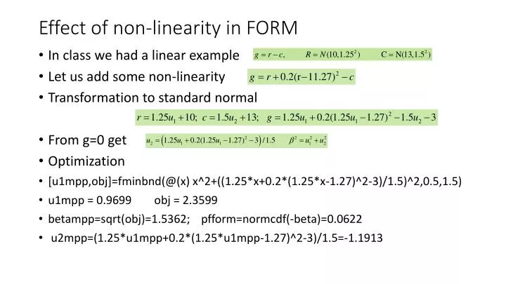
Effect of non-linearity in FORM • In class we had a linear example • Let us add some non-linearity • Transformation to standard normal • From g=0 get • Optimization • [u1mpp,obj]=fminbnd(@(x) x^2+((1.25*x+0.2*(1.25*x-1.27)^2-3)/1.5)^2,0.5,1.5) • u1mpp = 0.9699obj = 2.3599 • betampp=sqrt(obj)=1.5362; pfform=normcdf(-beta)=0.0622 • u2mpp=(1.25*u1mpp+0.2*(1.25*u1mpp-1.27)^2-3)/1.5=-1.1913
Visualization rmpp=u1mpp*1.25+10=11.2123 cmpp=1.5*u2mpp+13=11.2130 r=randn(1000,1)*1.25+10; c=randn(1000,1)*1.5+13; plot(r,c,'ro'); hold on g0=@(x) x+0.2.*(x-11.27).^2 fplot(g0,[5,15]) plot(rmpp,cmpp,'go','MarkerSize',15,'MarkerFaceColor','g') fplot(f,[5,15],'g'); xlabel('r');ylabel('c'); legend('samples','g=0','MPP','tangent','Location','SouthEast')
Check by MCS c=randn(1000000,1)*1.5+13; r=randn(1000000,1)*1.25+10; s=0.5*(sign(gs)+1); gs=r+0.2.*(r-11.27).^2-c; s=0.5*(sign(gs)+1); pf=sum(s)/1000000 =0.0811, 0.0806,0.0809 • Form 23% lower. • How much due to MCS error?
Example with uniform distributions • Let R=U(10,12), C=U(11,15), g=r-c. • To calculate the probability of failure we note that if • We start by an initial guess of normal variables with the same means and bounds corresponding to two standard deviations. • That is R’=N(11,0.52), C’=N(13,12)
Second iteration • For r: • normpdf(norminv(0.7))/0.5=0.6954 • For c:
General process for reliability index ur=(muc-mur)*sigr/sigc^2/(1+(sigr/sigc)^2) =0.9005 uc=(mur+sigr*ur-muc)/sigc=-0.9090 r=mur+sigr*ur=11.6615 c=muc+sigc*uc=11.6615 beta=sqrt(ur^2+uc^2)=1.2795 pf=normcdf(-beta)=0.1004