Search: complete architecture for intelligence? Search to solve the problem, “What to do?”

1. Review SearchThis material: Chapter 1-4 (3rd ed.)Read Chapter 13 (Quantifying Uncertainty) for ThursdayRead Chapter 18 (Learning from Examples) for next week • Search: complete architecture for intelligence? • Search to solve the problem, “What to do?” • Problem formulation: • Handle infinite or uncertain worlds • Search methods: • Uninformed, Heuristic, Local

2. Complete architectures for intelligence? • Search? • Solve the problem of what to do. • Learning? • Learn what to do. • Logic and inference? • Reason about what to do. • Encoded knowledge/”expert” systems? • Know what to do. • Modern view: It’s complex & multi-faceted.

3. Search?Solve the problem of what to do. • Formulate “What to do?” as a search problem. • Solution to the problem tells agent what to do. • If no solution in the current search space? • Formulate and solve the problem of finding a search space that does contain a solution. • Solve original problem in the new search space. • Many powerful extensions to these ideas. • Constraint satisfaction; means-ends analysis; etc. • Human problem-solving often looks like search.

4. Problem Formulation A problem is defined by four items: initial state e.g., "at Arad“ actions/transition model (3rd ed.) or successor function (2nd ed.) • Successor function: S(X) = set of states accessible from state X. • Actions(X) = set of actions available in State X • Transition Model: Result(S,A) = state resulting from doing action A in state S goal test, e.g., x = "at Bucharest”, Checkmate(x) path cost (additive) • e.g., sum of distances, number of actions executed, etc. • c(x,a,y) is the step cost, assumed to be ≥ 0 A solution is a sequence of actions leading from the initial state to a goal state

5. Vacuum world state space graph • states?discrete: dirt and robot location • initial state? any • actions?Left, Right, Suck • Transition Model or Successors as shown on graph • goal test?no dirt at all locations • path cost?1 per action

6. Vacuum world belief states: Agent’s belief about what state it’s in

7. Implementation: states vs. nodes • A state is a (representation of) a physical configuration • A node is a data structure constituting part of a search tree contains info such as: state, parent node, action, path costg(x), depth • The Expand function creates new nodes, filling in the various fields using the Successors(S) (2nd ed) or Actions(S) and Result(S,A)(3rd ed) of the problem.

8. Tree search algorithms • Basic idea: • Exploration of state space by generating successors of already-explored states (a.k.a.~expanding states). • Every generated state is evaluated: is it a goal state?

9. Tree search example

10. Repeated states • Failure to detect repeated states can turn a linear problem into an exponential one! • Test is often implemented as a hash table.

11. Solutions to Repeated States S B S • Graph search • never generate a state generated before • must keep track of all possible states (uses a lot of memory) • e.g., 8-puzzle problem, we have 9! = 362,880 states • approximation for DFS/DLS: only avoid states in its (limited) memory: avoid looping paths. • Graph search optimal for BFS and UCS, not for DFS. B C C C S B S State Space Example of a Search Tree optimal but memory inefficient

12. Search strategies • A search strategy is defined by picking the order of node expansion • Strategies are evaluated along the following dimensions: • completeness: does it always find a solution if one exists? • time complexity: number of nodes generated • space complexity: maximum number of nodes in memory • optimality: does it always find a least-cost solution? • Time and space complexity are measured in terms of • b: maximum branching factor of the search tree • d: depth of the least-cost solution • m: maximum depth of the state space (may be ∞)

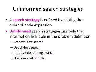
13. Uninformed search strategies • Uninformed: You have no clue whether one non-goal state is better than any other. Your search is blind. You don’t know if your current exploration is likely to be fruitful. • Various blind strategies: • Breadth-first search • Uniform-cost search • Depth-first search • Iterative deepening search (generally preferred) • Bidirectional search (preferred if applicable)

14. Breadth-first search • Expand shallowest unexpanded node • Frontier (or fringe): nodes in queue to be explored • Frontier is a first-in-first-out (FIFO) queue, i.e., new successors go at end of the queue. • Goal-Test when inserted. Is A a goal state?

15. Properties of breadth-first search • Complete?Yes it always reaches goal (if b is finite) • Time?1+b+b2+b3+… +bd + (bd+1-b)) = O(bd+1) (this is the number of nodes we generate) • Space?O(bd+1) (keeps every node in memory, either in fringe or on a path to fringe). • Optimal? Yes (if we guarantee that deeper solutions are less optimal, e.g. step-cost=1). • Space is the bigger problem (more than time)

16. Uniform-cost search Breadth-first is only optimal if path cost is a non-decreasing function of depth, i.e., f(d) ≥ f(d-1); e.g., constant step cost, as in the 8-puzzle. Can we guarantee optimality for any positive step cost? Uniform-cost Search: Expand node with smallest path cost g(n). • Frontier is a priority queue, i.e., new successors are merged into the queue sorted by g(n). • Remove successor states already on queue w/higher g(n). • Goal-Test when node is popped off queue.

17. Uniform-cost search Implementation: Frontier = queue ordered by path cost. Equivalent to breadth-first if all step costs all equal. Complete? Yes, if step cost ≥ ε (otherwise it can get stuck in infinite loops) Time? # of nodes with path cost ≤ cost of optimal solution. Space? # of nodes with path cost ≤ cost of optimal solution. Optimal? Yes, for any step cost ≥ ε

18. Depth-first search • Expand deepest unexpanded node • Frontier = Last In First Out (LIFO) queue, i.e., new successors go at the front of the queue. • Goal-Test when inserted. Is A a goal state?

19. Properties of depth-first search A • Complete? No: fails in infinite-depth spaces Can modify to avoid repeated states along path • Time?O(bm) with m=maximum depth • terrible if m is much larger than d • but if solutions are dense, may be much faster than breadth-first • Space?O(bm), i.e., linear space! (we only need to remember a single path + expanded unexplored nodes) • Optimal? No (It may find a non-optimal goal first) B C

20. Iterative deepening search • To avoid the infinite depth problem of DFS, we can • decide to only search until depth L, i.e. we don’t expand beyond depth L. •  Depth-Limited Search • What if solution is deeper than L?  Increase L iteratively. •  Iterative Deepening Search • As we shall see: this inherits the memory advantage of Depth-First • search, and is better in terms of time complexity than Breadth first search.

21. Properties of iterative deepening search • Complete? Yes • Time?O(bd) • Space?O(bd) • Optimal? Yes, if step cost = 1 or increasing function of depth.

22. Bidirectional Search • Idea • simultaneously search forward from S and backwards from G • stop when both “meet in the middle” • need to keep track of the intersection of 2 open sets of nodes • What does searching backwards from G mean • need a way to specify the predecessors of G • this can be difficult, • e.g., predecessors of checkmate in chess? • which to take if there are multiple goal states? • where to start if there is only a goal test, no explicit list?

23. Summary of algorithms Generally the preferred uninformed search strategy

24. Best-first search • Idea: use an evaluation functionf(n) for each node • f(n) provides an estimate for the total cost. • Expand the node n with smallest f(n). • g(n) = path cost so far to node n. • h(n) = estimate of (optimal) cost to goal from node n. • f(n) = g(n)+h(n). • Implementation: Order the nodes in frontier by increasing order of cost. • Evaluation function is an estimate of node quality • More accurate name for “best first” search would be “seemingly best-first search” • Search efficiency depends on heuristic quality

25. Heuristic function • Heuristic: • Definition: a commonsense rule (or set of rules) intended to increase the probability of solving some problem • “using rules of thumb to find answers” • Heuristic function h(n) • Estimate of (optimal) cost from n to goal • Defined using only the state of node n • h(n) = 0 if n is a goal node • Example: straight line distance from n to Bucharest • Note that this is not the true state-space distance • It is an estimate – actual state-space distance can be higher • Provides problem-specific knowledge to the search algorithm

26. Greedy best-first search • h(n) = estimate of cost from n to goal • e.g., h(n) = straight-line distance from n to Bucharest • Greedy best-first search expands the node that appears to be closest to goal. • f(n) = h(n)

27. Properties of greedy best-first search • Complete? • Tree version can get stuck in loops. • Graph version is complete in finite spaces. • Time?O(bm), but a good heuristic can give dramatic improvement • Space?O(bm) - keeps all nodes in memory • Optimal? No e.g., Arad  Sibiu  RimnicuVilcea  Pitesti  Bucharest is shorter!

28. A* search • Idea: avoid expanding paths that are already expensive • Evaluation function f(n) = g(n) + h(n) • g(n) = cost so far to reach n • h(n) = estimated cost from n to goal • f(n) = estimated total cost of path through n to goal • Greedy Best First search has f(n)=h(n) • Uniform Cost search has f(n)=g(n)

29. Admissible heuristics • A heuristic h(n) is admissible if for every node n, h(n) ≤ h*(n), where h*(n) is the true cost to reach the goal state from n. • An admissible heuristic never overestimates the cost to reach the goal, i.e., it is optimistic • Example: hSLD(n) (never overestimates the actual road distance) • Theorem: If h(n) is admissible, A* using TREE-SEARCH is optimal

30. Consistent heuristics(consistent => admissible) • A heuristic is consistent if for every node n, every successor n' of n generated by any action a, h(n) ≤ c(n,a,n') + h(n') • If h is consistent, we have f(n’) = g(n’) + h(n’) (by def.) = g(n) + c(n,a,n') + h(n’) (g(n’)=g(n)+c(n.a.n’)) ≥ g(n) + h(n) = f(n) (consistency) f(n’) ≥ f(n) • i.e., f(n) is non-decreasing along any path. • Theorem: If h(n) is consistent, A* using GRAPH-SEARCH is optimal It’s the triangle inequality ! keeps all checked nodes in memory to avoid repeated states

31. Contours of A* Search • A* expands nodes in order of increasing f value • Gradually adds "f-contours" of nodes • Contour i has all nodes with f=fi, where fi < fi+1

32. Properties of A* • Complete? Yes (unless there are infinitely many nodes with f ≤ f(G) , i.e. step-cost > ε) • Time/Space? Exponential except if: • Optimal? Yes (with: Tree-Search, admissible heuristic; Graph-Search, consistent heuristic) • Optimally Efficient: Yes (no optimal algorithm with same heuristic is guaranteed to expand fewer nodes)

33. Simple Memory Bounded A* • This is like A*, but when memory is full we delete the worst node (largest f-value). • Like RBFS, we remember the best descendent in the branch we delete. • If there is a tie (equal f-values) we delete the oldest nodes first. • simple-MBA* finds the optimal reachable solution given the memory constraint. • Time can still be exponential. A Solution is not reachable if a single path from root to goal does not fit into memory

34. SMA* pseudocode (not in 2nd edition 2 of book) function SMA*(problem) returns a solution sequence inputs: problem, a problem static: Queue, a queue of nodes ordered by f-cost Queue  MAKE-QUEUE({MAKE-NODE(INITIAL-STATE[problem])}) loop do ifQueue is empty then return failure n  deepest least-f-cost node in Queue if GOAL-TEST(n) then return success s NEXT-SUCCESSOR(n) if s is not a goal and is at maximum depth then f(s)   else f(s)  MAX(f(n),g(s)+h(s)) if all of n’s successors have been generated then update n’s f-cost and those of its ancestors if necessary if SUCCESSORS(n) all in memory then remove n from Queue if memory is full then delete shallowest, highest-f-cost node in Queue remove it from its parent’s successor list insert its parent on Queue if necessary insert s in Queue end

35. maximal depth is 3, since memory limit is 3. This branch is now useless. A A 12 13 A 0+12=12 10 8 B G B G 10+5=15 8+5=13 15 13 10 10 8 16 C D H I A A A 20+5=25 16+2=18 15[15] 15[24] 20[24] 20+0=20 A 8 10 10 8 8 15 B B G E F J K 15 20[] 24[] 30+5=35 30+0=30 24+0=24 24+5=29 B G I D 15 24 C 25 24 20 Simple Memory-bounded A* (SMA*) (Example with 3-node memory) Progress of SMA*. Each node is labeled with its currentf-cost. Values in parentheses show the value of the best forgotten descendant. best forgotten node best estimated solution so far for that node Search space g+h = f ☐ = goal A 13[15] A 12 G 13 B 15 18 H  24+0=24  Algorithm can tell you when best solution found within memory constraint is optimal or not.

36. Conclusions • The Memory Bounded A* Search is the best of the search algorithms we have seen so far. It uses all its memory to avoid double work and uses smart heuristics to first descend into promising branches of the search-tree.

37. Dominance • If h2(n) ≥ h1(n) for all n (both admissible) • then h2dominatesh1 • h2is better for search: it is guaranteed to expand less or equal nr of nodes. • Typical search costs (average number of nodes expanded): • d=12 IDS = 3,644,035 nodes A*(h1) = 227 nodes A*(h2) = 73 nodes • d=24 IDS = too many nodes A*(h1) = 39,135 nodes A*(h2) = 1,641 nodes

38. Relaxed problems • A problem with fewer restrictions on the actions is called a relaxed problem • The cost of an optimal solution to a relaxed problem is an admissible heuristic for the original problem • If the rules of the 8-puzzle are relaxed so that a tile can move anywhere, then h1(n) gives the shortest solution • If the rules are relaxed so that a tile can move to any adjacent square, then h2(n) gives the shortest solution

39. Effective branching factor • Effective branching factor b* • Is the branching factor that a uniform tree of depth d would have in order to contain N+1 nodes. • Measure is fairly constant for sufficiently hard problems. • Can thus provide a good guide to the heuristic’s overall usefulness.

40. Effectiveness of different heuristics • Results averaged over random instances of the 8-puzzle

41. Inventing heuristics via “relaxed problems” • A problem with fewer restrictions on the actions is called a relaxed problem • The cost of an optimal solution to a relaxed problem is an admissible heuristic for the original problem • If the rules of the 8-puzzle are relaxed so that a tile can move anywhere, then h1(n) gives the shortest solution • If the rules are relaxed so that a tile can move to any adjacent square, then h2(n) gives the shortest solution • Can be a useful way to generate heuristics • E.g., ABSOLVER (Prieditis, 1993) discovered the first useful heuristic for the Rubik’s cube puzzle

42. More on heuristics • h(n) = max{ h1(n), h2(n),……hk(n) } • Assume all h functions are admissible • Always choose the least optimistic heuristic (most accurate) at each node • Could also learn a convex combination of features • Weighted sum of h(n)’s, where weights sum to 1 • Weights learned via repeated puzzle-solving • Could try to learn a heuristic function based on “features” • E.g., x1(n) = number of misplaced tiles • E.g., x2(n) = number of goal-adjacent-pairs that are currently adjacent • h(n) = w1 x1(n) + w2 x2(n) • Weights could be learned again via repeated puzzle-solving • Try to identify which features are predictive of path cost

43. Local search algorithms • In many optimization problems, the path to the goal is irrelevant; the goal state itself is the solution • State space = set of "complete" configurations • Find configuration satisfying constraints, e.g., n-queens • In such cases, we can use local search algorithms • keep a single "current" state, try to improve it. • Very memory efficient (only remember current state)

44. Hill-climbing search • "Like climbing Everest in thick fog with amnesia"

45. Hill-climbing Difficulties • Problem: depending on initial state, can get stuck in local maxima

46. Gradient Descent • Assume we have some cost-function: • and we want minimize over continuous variables X1,X2,..,Xn • 1. Compute the gradient : • 2.Take a small step downhill in the direction of the gradient: • 3. Check if • 4. If true then accept move, if not reject. • 5. Repeat.

47. Simulated annealing search • Idea: escape local maxima by allowing some "bad" moves but gradually decrease their frequency

48. Properties of simulated annealing search • One can prove: If T decreases slowly enough, then simulated annealing search will find a global optimum with probability approaching 1 (however, this may take VERY long) • However, in any finite search space RANDOM GUESSING also will find a global optimum with probability approaching 1 . • Widely used in VLSI layout, airline scheduling, etc.

49. Tabu Search • A simple local search but with a memory. • Recently visited states are added to a tabu-list and are temporarily • excluded from being visited again. • This way, the solver moves away from already explored regions and • (in principle) avoids getting stuck in local minima.

50. Local beam search • Keep track of k states rather than just one. • Start with k randomly generated states. • At each iteration, all the successors of all k states are generated. • If any one is a goal state, stop; else select the k best successors from the complete list and repeat. • Concentrates search effort in areas believed to be fruitful. • May lose diversity as search progresses, resulting in wasted effort.