Download
1 / 19
190 likes | 212 Views
Explore how nearest-neighbor imputation and Landsat time series can enhance monitoring of late-successional forest habitat across large regions, providing detailed trend information. Preliminary results and challenges are discussed.

E N D
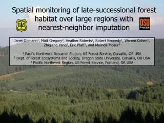
Spatial monitoring of late-successional forest habitat over large regions with nearest-neighbor imputation Janet Ohmann1, Matt Gregory2, Heather Roberts2, Robert Kennedy2, Warren Cohen1, Zhiqiang Yang2, Eric Pfaff2, and Melinda Moeur3 1 Pacific Northwest Research Station, US Forest Service, Corvallis, OR USA 2 Dept. of Forest Ecosystems and Society, Oregon State University, Corvallis, OR USA 3 Pacific Northwest Region, US Forest Service, Portland, OR USA
Needs for regional vegetation information • Complexity and scope of current forest issues (sustainability, climate change, etc.) are pushing technology to provide information that is: • Consistent over large regions, detailed forest attributes, spatially explicit (mapped)... with trend information (monitoring) • Can we marry two current technologies to better meet needs? • Nearest-neighbor imputation (detailed attributes) • Change detection from Landsat time series (trends) • Approach: minimize sources of error in two model dates, map real change
Northwest Forest Plan of 1994 • Conservation plan for older forests and species on federal lands • Effectiveness Monitoring: • Develop maps for assessing change in older forest and habitat, 1996 to 2006 Provinces (23 mill. ha.) USA
Regional inventories: unbalanced in space and time • Choose one plot per location • Match to closest (96 or 06) imagery date • Develop single gradient model with all plots • Apply model to each imagery year • Imagery is only source of change (gradient model, plot sample, and other GIS layers held constant) Imagery years
Landsat Detection of Trends in Disturbance and Recovery (LandTrendr)* • Normalizes across time-series at pixel level • Change ‘trajectories’ describe sequences of disturbance, regrowth • Frequent time-steps • Detect gradual and subtle changes • ‘Temporally normalized’ imagery for multi-year GNN *Kennedy et al. (in press), Rem. Sens. Env.
Defining ‘late-successional and old growth’ (LSOG) forest • Simple definition for this analysis: • QMD > 50 cm • > 10% canopy cover • Compute from tree-level data, associate with GNN pixels • Ideally, ecological definition (index based on multiple components): • Large, old live trees • Large snags • Large down wood • Multi-layered canopy
Aggregate change in older forest (LSOG) at regional level • Slight net loss (33.2% to 32.5%) • 3% of 1996 LSOG lost, mostly to large wildfires, partially offset by regrowth in other areas • Over 10 years, net change signal is swamped by noise Based on LSOG % correct from cross-validation
Not LSOG LSOG gain LSOG loss LSOG Nonforest Spatial change in Klamath province, 1996-2006 • Change is dramatic in some landscapes (2002 Biscuit Fire) • Spatial change is quite noisy
Not LSOG LSOG gain LSOG loss LSOG Nonforest Spatial change at landscape level 2006 Landtrendr B-G-W 1996 Landtrendr B-G-W GNN change
Pixel-level noise in GNN models • GNN with k=1 is inherently noisy: sensitive to slight spectral shifts • Minor changes cause plots to cross definition threshold (QMD) • Problems magnified by model ‘subtraction’ (spatial predictors, plot sampling and location errors, model specification, etc.) • GNN cross-validation applies to 2-date ‘hybrid’ model, not spatial change All plots 1991-2008
How reliable is spatial change from two GNN models? • What is truth? No data available for validating spatial change. • Corroborates other estimates: • Plot-based estimates from FIA Annual inventory • Within 1% of previous 1996 estimate (different methods) • Slight net loss corroborated by remeasured plots • A different approach to validation is needed... FIA Annual plots 2001-2008 Oregon Western Cascades
TimeSync validation(Cohen et al. in press, RSE) • Expert interpretation of Landsat time series and ancillary data 1998 2005
Adapting TimeSync to validation of GNN change (1996-2006) Confusion matrices: Data recording in TimeSync:
Lessons learned: multi-temporal GNN for monitoring • Only feasible with “temporally normalized” imagery • Net change over large spatial extents is reasonable • More work to quantify our ability to map pixel-level change • 10 years is insufficient to reliably map ‘ingrowth’ of older forest, but loss from disturbance is feasible
Improvements coming soon... • Yearly matching of plots to imagery • Prior disturbance and growth (from LandTrendr) informs model Disturbance Magnitude (1996 to 2006) Imagery years
Normalized Landsat mosaics (Remote Sensing Applications Center, USFS) 1996 2006 1996 B-G-W 2006 B-G-W • GNN QMD “change” • (bias associated with aspect) 1996 GNN QMD 2006 GNN QMD