CONDITIONAL PROBABILITY AND RELEVANCE
CONDITIONAL PROBABILITY AND RELEVANCE. Conditional Relative Frequency. Two-Way Frequency Tables

CONDITIONAL PROBABILITY AND RELEVANCE
E N D
Presentation Transcript
CONDITIONAL PROBABILITY AND RELEVANCE Probability and Statistics for Teachers, Math 507, Lecture 4
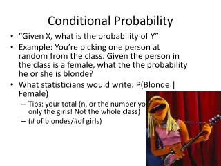
Conditional Relative Frequency • Two-Way Frequency Tables • An Example of a 2x2 frequency table: This table categorizes students at a medium-sized college in two ways. The categories in the top row must partition the population/sample space S and the categories in the first column must do the same. That is they must be disjoint and their union must be the whole set S. In other words, every member of the population must fall into exactly one category. In this case every student is either in F or in U but not both, and each is in P or in G but not both. The entries in the body of the table are the counts (frequencies) of elements falling in the intersection of the groups in the corresponding row and column. For instance, 600 students are in the intersection of P and F. The marginal numbers are totals of their rows or columns. The lower right corner is the size of S itself. Probability and Statistics for Teachers, Math 507, Lecture 4
Conditional Relative Frequency • Two-Way Frequency Tables • An Example of a 3x4 frequency table: Here is the same data partitioned more finely. Notice that the categories across the top still partition the data as do the categories down the first column. Probability and Statistics for Teachers, Math 507, Lecture 4
Conditional Relative Frequency • Two-Way Relative Frequency Tables • To turn a two-way frequency table into a two-way relative frequency table (also called a contingency table), divide every number in the table by the total number of elements in the population/sample space. In the two examples above, this means divide every number by 5000. Thus every number becomes a fraction between 0 and 1 (that should sound familiar) indicating the percentage of S falling in that intersection of categories. The number in the lower right-hand corner should always be 1. Probability and Statistics for Teachers, Math 507, Lecture 4
Conditional Relative Frequency • Two-Way Relative Frequency Tables • Example of a 2x2 relative frequency table: Here is the table we saw before, converted into a relative frequency table. It tells us that, for instance, 52% of students at the college are upperclassmen in good standing and 40% are freshmen. Probability and Statistics for Teachers, Math 507, Lecture 4
Conditional Relative Frequency • Two-Way Relative Frequency Tables • Example of a 3x4 relative frequency table: Here is the other table we saw before, converted to a relative frequency table. Here we see that 2.4% of the students are juniors with honors and 1% are seniors on probation. Probability and Statistics for Teachers, Math 507, Lecture 4
Conditional Relative Frequency • The values in the two previous tables are observed relative frequencies. If we let S be the population of students at the college and P be the proportion of students falling into each subset, then P is a probability measure on S, several of whose values appear in the relative frequency tables. For instance, P(G)=0.80, P(FR)=0.40, , and Probability and Statistics for Teachers, Math 507, Lecture 4
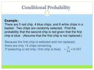
Conditional Relative Frequency • Suppose we want to know the proportion of freshmen among students on probation. That is, if we look only at students on probation, what proportion of them are freshmen. Since there are 1000 students on probation and 600 of them are freshmen, then the proportion of freshmen among students on probation is 0.60. We denote this quantity by P(FR|P) and call it the “fraction of FR among P” or the “conditional relative frequency of FR in P” or the “conditional (empirical) probability of FR given P.” As a formula, then, Probability and Statistics for Teachers, Math 507, Lecture 4
Conditional Relative Frequency • In the previous formula, if we divide numerator and denominator by |S|, we see that we can get conditional relative frequency simply by knowing the values of the probability measure: • In general for events A and B we will define the conditional relative frequency of A in B by Probability and Statistics for Teachers, Math 507, Lecture 4
Conditional Relative Frequency • Note that P(FR)=0.40 but P(FR|P)=0.60. So P(FR|P)>P(FR). That is, the proportion of freshmen among students on probation is greater than the proportion of freshmen in the whole student population. We can say that freshmen are overrepresented among the students on probation. Similarly while P(P)=0.20. That is, 30% of freshmen are on probation while only 20% of the student population is on probation. So P(P|FR)>P(FR) and we can say that students on probation are overrepresented among freshmen. It turns out that one overrepresentation implies the other: if A is overrepresented in B, then B is always represented in A. (The same holds for underrepresentation and proportional representation, discussed below). Probability and Statistics for Teachers, Math 507, Lecture 4
Conditional Relative Frequency • Given events A and B, if P(A|B)<P(A), then A is underrepresented in B. In that case it also holds that P(B|A)<P(B); that is, B is underrepresented in A. As an example, P(SE)=0.16 but P(SE|P)=0.01/0.20=0.05; seniors are 16% of the student population but only 5% of the students on probation, so seniors are underrepresented among the students on probation. It will follow from a future theorem that probationary students are also underrepresented among seniors. We can verify this particular case by noting P(P)=0.20 but P(P|SE)=0.01/0.16=0.0625, so P(P)<P(P|SE). Twenty percent of students are on probation, but only 6.25% of seniors are. Probability and Statistics for Teachers, Math 507, Lecture 4
Conditional Relative Frequency • Further, for events A and B, if P(A|B)=P(A), then we say that A is proportionally represented in B. (Again this also implies B is proportionally represented in A). The above table does not seem to offer an example of proportional representation, but the table and discussion at the top of page 34 do. Probability and Statistics for Teachers, Math 507, Lecture 4
Conditional Probability • More generally, if A and B are events in some sample space S, and P is a probability measure on S, then we define (assuming P(B) is not zero), the conditional probability of A given B. This differs from the previous discussion only in that P is not necessarily observed relative frequency. Probability and Statistics for Teachers, Math 507, Lecture 4
Conditional Probability • For example suppose we roll a fair die. Then S={1,2,3,4,5,6} and P is the uniform probability measure. Let A be the event “the roll is even” and B be the event “the roll is greater than three.” Then the conditional probability of an even roll given a roll greater than three is P(A|B)=P(roll even and >3)/P(roll >3) =P({4,6})/P({4,5,6})=(2/6)/(3/6)=2/3. • Compare this to P(A)=P({2,4,6})=3/6=1/2. Probability and Statistics for Teachers, Math 507, Lecture 4
Conditional Probability • One way of viewing conditional probability is as a revision of probabilities assessed prior to any knowledge about the outcome. In the previous example, the prior probability of an even roll is P(A)=1/2. If we happen to learn that the roll was greater than three, then we revise the probability of an even roll to the conditional probability P(A|B)=2/3. That is, knowledge that the roll exceeds three increases the probability that the roll is even. Probability and Statistics for Teachers, Math 507, Lecture 4
Conditional Probability • Under these circumstances (that is, P(A|B)>P(A)) we say that B is positively relevant to A since knowledge that B happens increases the likelihood that A happens. This is the same as saying A is overrepresented in B, but we change the terminology to reflect the possibility that P is a theoretical probability rather than an experimental one. Similarly, if P(A|B)<A, then B is negatively relevant to A, and if P(A|B)=A then B is independent of (or irrelevant to) A. Probability and Statistics for Teachers, Math 507, Lecture 4
Conditional Probability • For instance suppose you roll two dice, one red and one clear. Define events A=”roll a sum of 10” and B=”roll a sum of 7” and C=”the clear die rolls 2”. Then P(A)=3/36=1/12 and P(A|C)=0, so C is negatively relevant to A. This says that a sum of 10 becomes less likely (indeed impossible in this case!) if the clear die is known to be 2. • Also P(B)=6/36=1/6 and P(B|C)=1/6, so B and C are independent. This says that the probability of rolling a sum of 7 is unchanged by the knowledge that the clear die is a 2. Probability and Statistics for Teachers, Math 507, Lecture 4
Conditional Probability • Theorem 2.5: Given a sample space S with probability measure P and fixed event B, the conditional probability of events given B is itself a probability measure. That is, conditional probabilities are between 0 and 1, the conditional probabilities of the empty set and the sample space are 0 and 1 respectively, the conditional probability of a disjoint union is the sum of the conditional probabilities of the individual events, and the same is true for countable unions of pairwise disjoint events. The book lists these conditions formally in expressions 2.29, 2.30, 2.31, and 2.32 on page 36 and proves the theorem. The concise summary of the theorem is conditional probability is probability. Probability and Statistics for Teachers, Math 507, Lecture 4
Relevance and Independence • Theorem 2.6 (the proof is in the book): Let S be a sample space with probability measure P, and let A and B be events in S. Then all of the following conditions are equivalent, all indicating that B is positively relevant for A. Probability and Statistics for Teachers, Math 507, Lecture 4
Relevance and Independence • Example: Consider again the events A=”the roll is even” and B=”the roll exceeds three” in the experiment that consists of rolling a single die. Then note how each of the four conditions is satisfied. • P(A|B)=2/3 > P(A)=1/2. • , and Probability and Statistics for Teachers, Math 507, Lecture 4
Relevance and Independence • Theorem 2.8: The conditions in theorem 2.6 are also equivalent if all greater than symbols are replaced by less than symbols. In that case they all indicate negative relevance of B for A. • Theorem 2.10: The conditions in theorem 2.6 are also equivalent if all greater than symbols are replaced by equal signs. In that case they all indicate independence of A and B. Probability and Statistics for Teachers, Math 507, Lecture 4
Relevance and Independence • Theorems 2.7, 2.9, and 2.11 prove that if B is positively relevant for, negatively relevant for, or independent of A, then A holds the same relationship to B. Most probability texts define A and B to be independent if and we will frequently use this equation as our test for independence. Probability and Statistics for Teachers, Math 507, Lecture 4
Relevance and Independence • The book mentions yet another condition equivalent to positive relevance, negative relevance, or independence. It involves testing the determinant of the 2x2 matrix whose entries are those of the two-way table whose categories are A, the complement of A, B, and the complement of B. Probability and Statistics for Teachers, Math 507, Lecture 4
Statistical Highlight: Simpson’s Paradox • In 1999 at the University of Calizona at Los Phoenix (UCLP), 393 men applied to the graduate school and 294 were admitted for an admission rate of 74.8%. The same year 444 women applied and 135 were admitted for an admission rate of 30.4%. To UCLP administrators this strongly suggested sex bias favoring men in graduate admissions. To track down the source of the bias, administrators ordered the individual graduate programs at UCLP to report their admission rates for men and women in 1999. This was a simple task in that UCLP has graduate programs in only four fields: English, Physics, Psychology, and Materials Science. Probability and Statistics for Teachers, Math 507, Lecture 4
Statistical Highlight: Simpson’s Paradox • Below is a table giving the results of the investigation. Note carefully which of the four departments admit men at higher rates than women. Probability and Statistics for Teachers, Math 507, Lecture 4
Statistical Highlight: Simpson’s Paradox • The baffled administration at UCLP is at a loss to explain the situation. Every department admits women at a higher rate than men, but overall the university admits men at a much higher rate than women. This counterintuitive situation is a concrete example of Simpson’s Paradox. This paradox asserts that event A may be positively relevant to event B in every block of some partition of the population and yet be negatively relevant in the population as a whole (e.g., being female is positively relevant to being admitted in every program yet negatively relevant to being admitted overall). Probability and Statistics for Teachers, Math 507, Lecture 4
Statistical Highlight: Simpson’s Paradox • In our example the source of the problem is clear. The two departments that have low admission rates overall also have high numbers of applications from women and low numbers from men. In the two departments with high admission rates overall the situation is reversed. Thus a large percentage of men are admitted and a large percentage of women are not, even though every department admits women at a higher rate than men. Probability and Statistics for Teachers, Math 507, Lecture 4
Statistical Highlight: Simpson’s Paradox • Here are some other scenarios in which Simpson’s Paradox might arise: • Baseball player Willie may have a higher batting average than player Hank every year of their careers, and yet Hank may have the higher lifetime batting average. • Cancer treatment A may produce a higher recovery rate than treatment B at every hospital in which both are tested, and yet treatment B may have the higher overall recovery rate when the data are combined. Probability and Statistics for Teachers, Math 507, Lecture 4
Statistical Highlight: Simpson’s Paradox • Examples of Simpson’s Paradox occur in real life. One famous example appears in the paper “Sex Bias in Graduate Admissions: Data from Berkeley,” in Science 187 (Feb. 1975), pp. 398–404, by Bickel, Hammel, and O’Connell. In that case the data was not quite unidirectional (that is, there were some departments that admitted men at higher rates than women), yet the overall picture is still a toned-down version of our fictitious example above. Probability and Statistics for Teachers, Math 507, Lecture 4
Statistical Highlight: Simpson’s Paradox • More elaborate versions of Simpson’s paradox are possible in which the flip-flopping of positive to negative relevance happens multiple times. For example Willie can have a higher batting average than Hank in every ballpark in every year; Hank can have the higher overall batting average for each year; and yet Willie can have the higher lifetime average. Again, cancer treatment A can produce the higher recovery rate in every hospital; B can produce the higher recovery rate in every state (combining the data from each hospital in the state); yet A can have the higher national recovery rate. Examples are not too hard to manufacture, but a good spreadsheet helps! Probability and Statistics for Teachers, Math 507, Lecture 4
Statistical Highlight: Simpson’s Paradox • Here is a double flip-flop on cancer treatments. Probability and Statistics for Teachers, Math 507, Lecture 4