Download
1 / 36
360 likes | 520 Views
Branch statistics. Branches occur every 4-7 instructions on average in integer programs, commercial and desktop applications; somewhat less frequently in scientific ones Unconditional branches : 20% (of branches) Conditional (80%)

E N D
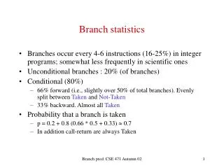
Branch statistics • Branches occur every 4-7 instructions on average in integer programs, commercial and desktop applications; somewhat less frequently in scientific ones • Unconditional branches : 20% (of branches) • Conditional (80%) • 66% forward (i.e., slightly over 50% of total branches). Most often Not Taken • 33% backward. Almost all Taken • Probability that a branch is taken • p = 0.2 + 0.8 (0.66 * 0.4 + 0.33) 0.6 (in fact simulations show a little less than that) • In addition call-return are always Taken Branch Prediction CSE 471
Conditional Branches • When do you know you have a branch? • During ID cycle (Could you know before that?) • When do you know if the branch is Taken or Not-Taken • During EXE cycle (e.g., for the MIPS) • Need for sophisticated solutions because • Modern pipelines are deep (could be more than 10 stages between ID and EXE) • Several instructions issued/cycle (compounds the “number of issueinstruction slots” being lost) • Several predicted branches in-flight at the same time Branch Prediction CSE 471
Misprediction Penalties Branch Prediction CSE 471
Inter-branch Latencies(data from Jimenez SPEC2000 simulation of 4-issue processor) Branch Prediction CSE 471
Anatomy of a Branch Predictor All instructions (BTB) Branch inst. (BPB) PC and/or global history and/or local history Prog. Exec. Event selec. Pred. Index. One level (BPB) Two level (History +PHT) Decoupled BTB + BPB Recovery? Feedback Pred. Mechan. Static (ISA) 1 or 2-bit saturating counters Markov Predictors Branch outcome Update pred. mechanism Update history (updates might be speculative) Branch Prediction CSE 471
Simple schemes to handle branches • Techniques that could work for CPU’s with a single pipeline with few stages are not practical for deep pipelines • Predictions are required • Static schemes (only software): not precise enough • Dynamic schemes: hardware assists Branch Prediction CSE 471
Simple static predictive schemes • Predict branch Not -Taken (easiest to implement; default for dynamic branch prediction) • If prediction correct no problem; • If prediction incorrect, delay = number of stages between ID and EXE • Predict branch Taken • Interesting only if target address can be computed early • Prediction depends on the direction of branch • Backward-Taken-Forward-Not-Taken (BTFNT) • Rationale: Backward branches at end of loops: mostly taken Branch Prediction CSE 471
Dynamic branch prediction • Execution of a branch requires knowledge of: • There is a branch but one can surmise that every instruction is a branch for the purpose of guessing whether it will be taken or not taken (i.e., prediction can be done at IF stage) • Whether the branch is Taken/Not-Taken (hence a branch prediction mechanism) • If the branch is taken what is the target address (can be computed but can also be “precomputed”, i.e., stored in some table) • If the branch is taken what is the instruction at the branch target address(saves the fetch cycle for that instruction) Branch Prediction CSE 471
Basic idea • Use a Branch Prediction Buffer (BPB) • Also called Branch Prediction Table (BPT), Branch History Table (BHT) • Records previous outcomes of the branch instruction • How it will be indexed, updated etc. see later • A prediction using BPB is attempted when the branch instruction is fetched (IF stage or equivalent) • It is acted upon during ID stage (when we know we have a branch) Branch Prediction CSE 471
Prediction Outcomes • Has a prediction been made (Y/N) • If not use default “Not Taken” • Is it correct or incorrect • Two cases: • Case 1: Yes and the prediction was correct (known at EXE stage) or No but the default was correct: No delay • Case 2: Yes and the prediction was incorrect or No and the default was incorrect: Delay Branch Prediction CSE 471
Simplest design • BPB addressed by lower bits of the PC • One bit prediction • Prediction = direction of the last time the branch was executed • Will mispredict at first and last iterations of a loop • Known implementation • Alpha 21064. The 1-bit table is associated with an I-cache line, one bit per line (4 instructions) Branch Prediction CSE 471
Improve prediction accuracy (2-bit saturating counter scheme)Property: takes two wrong predictions before it changes T to NT (and vice-versa) taken ^ Generally, this is the initial state not taken predict taken predict taken taken taken not taken not taken predict not taken predict not taken taken ^ not taken Branch Prediction CSE 471
Two bit saturating counters • 2 bits scheme used in: • Alpha 21164, UltraSparc, Pentium, Power PC 604 and 620 with variations, MIPS R10000 etc... • PA-8000 uses a variation • Majority of the last 3 outcomes (no state machine, just a shift register) • Why not 3 bit (8 states) saturating counters? • Performance studies show it’s not that worthwhile although it is present in the Alpha 21264 Branch Prediction CSE 471
Branch Prediction Buffers • Branch Prediction Buffer (BPB) • How addressed (low-order bits of PC, hashing, cache-like) • How much history in the prediction (1-bit, 2-bits, n-bits) • Where is it stored (in a separate table, associated with the I-cache) • Correlated branch prediction • 2-level prediction (keeps track of other branches) • Branch Target Buffers (BTB) • BPB + address of target instruction (+ target instruction -- not implemented in current micros as far as I know--) • Hybrid predictors • Choose dynamically the best among 2 predictors Branch Prediction CSE 471
Variations on BPB design Table of counters (predictions) often called PHT (pattern history table) Tag Counters Simple indexing (drawback “aliasing”) Cache-like (drawback: expensive) PC PC Branch Prediction CSE 471
Where to put the BPB • Associated with I-cache lines • 1 counter/instruction: Alpha 21164 • 2 counters/cache line (1 for every 2 instructions) : UltraSparc • 1 counter/cache line (AMD K5) • Separate table with cache-like tags in general with BTB’s (see in a few slides) • direct mapped : 512 entries (MIPS R10000), 1K entries (Sparc 64), 2K + BTB (PowerPC 620) • 4-way set-associative: 256 entries BTB (Pentium) • 4-way set-associative: 512 entries BTB + “2-level”(Pentium Pro) Branch Prediction CSE 471
Performance and Feedback of BPB’s • Prediction accuracy is only one of several metrics • Misfetch(correct prediction but time to compute the address; e.g. for unconditional branches or T/T if no Branch Target Buffer) • Mispredict(incorrect branch prediction) • These penalties might need to be multiplied by the number of instructions that could have been issued • Need to update PHT when direction has been determined • A potential problem: The same branch predicted several times before reaching decision on direction (tight loops) Branch Prediction CSE 471
Prediction accuracy • 2-bit vs. 1-bit • Significant gain: approx. 92% vs. 85% for f-p in Spec benchmarks, 90% vs. 80% in gcc but about 88% for both in compress • Table size and organization • The larger the table, the better (in general) but seems to max out at about 1K entries • Larger associativity if cache-like design improves accuracy (in general) Branch Prediction CSE 471
Correlated or 2-level branch prediction • Outcomes of consecutive branches are not independent • Classical example loop …. if ( x = = 2) /* branch b1 */ x = 0; if ( y = = 2) /* branch b2 */ y = 0; if ( x != y) /* branch b3 */ do this else do that Branch Prediction CSE 471
What should a good predictor do? • In previous example if both b1 and b2 are Taken, b3 should be Not-Taken • A two-bit counter scheme cannot predict this behavior. • Needs history of previous branches hence correlated schemes for BPB’s • Requires history of n previous branches (shift register) • Use of this vector (maybe more than one) to index a Pattern History Table (PHT) (maybe more than one) Branch Prediction CSE 471
General idea: implementation using a global history register and a global PHT PHT k 2 entriesof 2-bit counters t t nt t nt nt Global historyregister last k branches (t =1, nt =0) Branch Prediction CSE 471
Gshare: a popular predictor PHT The Global history register and selected bits of the PC are XORed to provide the index in a single PHT The idea is to try and avoid aliasing, i.e. avoid interference for two different branches with the same pattern Global history register XOR PC Branch Prediction CSE 471
Classification of 2-level (correlated) branch predictors • How many global registers and their length: • GA: Global (one) • PA: One per branch address (Local) (motivation: end of loop) • SA: Group several branch addresses • How many PHT’s: • g: Global (one) • p : One per branch address • s: Group several branch addresses • Previous slide was GAg (6,2) • The “6” refers to the length of the global register • The “2” means we are using 2-bit counters Branch Prediction CSE 471
Two level Global predictors p (or s) one PHT per address or set of addresses PC g GA GA GAg (5,2) GAp(5,2) Branch Prediction CSE 471
Two level per-address predictors p (or s) one PHT per address or set of addresses One global PHT g History (shift) registers; one per address History (shift) registers; one per address PC PC PAg (4,2) PAp(4,2) Branch Prediction CSE 471
Evaluation • The more hardware (real estate) the better! • GA s for a given number of “s” the larger G the better; for a given “G” length, the larger the number of “s” the better. • SAg with a limited number of registers performs better than gshare at same PHT size (used in Pentium III and Pentium 4) • Note that the result of a branch might not be known when the GA (or PA) needs to be used again. It must be speculatively updated (and repaired if need be) • Why? How (hint: checkpoint history registers)? • Ditto for PHT but less in a hurry? Branch Prediction CSE 471
Branch Target Buffers • BPB: Tag (not always) + Prediction • BTB: Tag + prediction + next address • Now we predict and “precompute” branch outcome and target address during IF • Of course more costly • Can still be associated with cache line (UltraSparc) • Implemented in a straightforward way in Pentium; not so straightforward in Pentium Pro, III and 4 (see later) • Decoupling (see later) of BPB and BTB in Power PC and PA-8000 • Entries put in BTB only on taken branches (small benefit) Branch Prediction CSE 471
BTB layout 2-bit counter or local history register + PHT Target instruction address or I-cache line target address Tag cache-like (Partial) PC Next PC (target address) Prediction During IF, check if there is a hit in the BTB. If so, the instruction must be a branch and we can get the target address – if predicted taken – during IF. If correct, no stall Branch Prediction CSE 471
The “Misfetch” Misprediction in BTB • Correct “Taken” prediction but incorrect target address • Resolved after decode during target address computation • Can happen for “return” (but see later) • Can happen for “indirect jumps” (rare but costly) • Might have become more frequent in object-oriented programming such as C++, Java Branch Prediction CSE 471
Decoupled BPB and BTB • For a fixed real estate (i.e., fixed area on the chip): • Increasing the number of entries implies less bits for history (important if the prediction is two-level) • Increasing the number of entries implies better accuracy of prediction. • Decoupled design • Separate – and different sizes – BPB and BTB • BPB. If it predicts taken then go to BTB (see next slide) • Power PC 620: 2K entries BPB + 256 entries BTB • HP PA-8000: 256*3 BPB + 32 (fully-associative) BTB Branch Prediction CSE 471
Decoupled BTB BPB Tag Hist BTB (2) access BPB or any 2-level predictor Tag Next address (3) if match and prediction is T then set PC to target address Note: the BPB does not require a tag, so could be much larger (1) Access BTB PC Branch Prediction CSE 471
Return jump stack • Indirect jumps difficult to predict except returns from procedures (but luckily returns are about 85% of indirect jumps) • If returns are entered with their target address in BTB, most of the time it will be the wrong target • Procedures are called from many different locations • Hence addition of a small “return stack”; 4 to 8 entries are enough (1 in MIPS R10000, 4 in Alpha 21064, 4 in Sparc64, 12 in Alpha 21164) • Checked during IF, in parallel with BTB. Branch Prediction CSE 471
Resume buffer • In some “old” machines (e.g., IBM 360/91 circa 1967), branch prediction was implemented by fetching both paths (limited to 1 branch) • Similar idea: “resume buffer” in MIPS R10000. • If branch predicted taken, it takes one cycle to compute and fetch the target • During that cycle save the Not-Taken sequential instruction in a buffer (4 entries of 4 instructions each). • If mispredict, reload from the “resume buffer” thus saving one cycle Branch Prediction CSE 471
Hybrid Predictor (schematic) The green, red, and blue arrows might correspond to different indexing functions. P1 (e.g., local PHT) P2(e.g.,gshare) P1c/P2c Selects which predictor to use (e.g. tournament predictor) PC Global Branch Prediction CSE 471
Tournament Predictor 0/0, 1/0, 1/1 0/0, 0/1, 1/1 Use Pred 1 Use Pred 2 0/1 1/0 1/0 0/1 0/1 Use Pred 1 Use Pred 2 1/0 0/0,1/1 0/0,1/1 0: pred is incorrect; 1 pred is correct; a/b pred for Pred 1 / Pred 2 Branch Prediction CSE 471
Performance • Hybrid predictor consisting of a local predictor of size s1 and a global predictor of size s2 seems to perform better than a local or global predictor of size s s1 + s2 • Use machine learning (AI) techniques? • Start with a “quick and dirty” predictor yielding a prediction in one cycle • Concurrently use a slower, more accurate predictor. If its prediction disagrees with the fast predictor, roll back the computation. Branch Prediction CSE 471