Download
1 / 36
360 likes | 478 Views
CS 140 : Matrix multiplication. Linear algebra problems Matrix multiplication I : cache issues Matrix multiplication II: parallel issues Thanks to Jim Demmel and Kathy Yelick (UCB) for some of these slides. Problems in linear algebra. Solving linear equations:

E N D
CS 140 : Matrix multiplication • Linear algebra problems • Matrix multiplication I : cache issues • Matrix multiplication II: parallel issues Thanks to Jim Demmel and Kathy Yelick (UCB) for some of these slides
Problems in linear algebra • Solving linear equations: • Find x such that A*x = b • Workhorse of computational modeling • Dense: electromagnetics; kernel in sparse • Sparse: differential equations, etc. • Eigenvalue / eigenvector: • Find λand xsuch that A*x = λ*x • Dynamics of systems; vibration; information retrieval • Today: Matrix – matrix multiplication • Compute C = A * B • Kernel in linear equation solvers, etc.
Sequential Matrix Multiplication Simple mathematics, but getting good performance is complicated by memory hierarchy --- cache issues.
Avoiding data movement: Reuse and locality Conventional Storage Hierarchy Proc Proc Proc • Large memories are slow, fast memories are small • Parallel processors, collectively, have large, fast cache • the slow accesses to “remote” data we call “communication” • Algorithm should do most work on local data Cache Cache Cache L2 Cache L2 Cache L2 Cache L3 Cache L3 Cache L3 Cache potential interconnects Memory Memory Memory
Simplified model of hierarchical memory • Assume just 2 levels in the hierarchy, fast and slow • All data initially in slow memory • m = number of memory elements (words) moved between fast and slow memory • tm = time per slow memory operation • f = number of arithmetic operations • tf = time per arithmetic operation << tm • q = f / m average number of flops per slow element access • Minimum possible time = f* tf when all data in fast memory • Actual time • f * tf + m * tm = f * tf * (1 + tm/tf * 1/q) • Larger q means time closer to minimum f * tf
“Naïve” Matrix Multiply {implements C = C + A*B} for i = 1 to n for j = 1 to n for k = 1 to n C(i,j) = C(i,j) + A(i,k) * B(k,j) Algorithm has 2*n3 = O(n3) Flops and operates on 3*n2 words of memory A(i,:) C(i,j) C(i,j) B(:,j) = + *
Matrix Multiply on RS/6000 12000 would take 1095 years T = N4.7 Size 2000 took 5 days O(N3) performance would have constant cycles/flop Performance looks much closer to O(N5) Slide source: Larry Carter, UCSD
Matrix Multiply on RS/6000 Page miss every iteration TLB miss every iteration Cache miss every 16 iterations Page miss every 512 iterations Slide source: Larry Carter, UCSD
“Naïve” Matrix Multiply {implements C = C + A*B} for i = 1 to n {read row i of A into fast memory} for j = 1 to n {read C(i,j) into fast memory} {read column j of B into fast memory} for k = 1 to n C(i,j) = C(i,j) + A(i,k) * B(k,j) {write C(i,j) back to slow memory} A(i,:) C(i,j) C(i,j) B(:,j) = + *
“Naïve” Matrix Multiply How many references to slow memory? m = n3 read each column of B n times + n2 read each row of A once + 2n2 read and write each element of C once = n3 + 3n2 So q = f / m = 2n3 / (n3 + 3n2) ~= 2 for large n, no improvement over matrix-vector multiply A(i,:) C(i,j) C(i,j) B(:,j) = + *
Blocked Matrix Multiply Consider A,B,C to be N by N matrices of b by b subblocks where b=n / N is called the block size for i = 1 to N for j = 1 to N {read block C(i,j) into fast memory} for k = 1 to N {read block A(i,k) into fast memory} {read block B(k,j) into fast memory} C(i,j) = C(i,j) + A(i,k) * B(k,j) {do a matrix multiply on blocks} {write block C(i,j) back to slow memory} A(i,k) C(i,j) C(i,j) = + * B(k,j)
Blocked Matrix Multiply m is amount memory traffic between slow and fast memory matrix has nxn elements, and NxN blocks each of size bxb f is number of floating point operations, 2n3 for this problem q = f / m measures algorithm efficiency in the memory system m = N*n2 read a block of B N3 times (N3 * n/N * n/N) + N*n2 read a block of A N3 times + 2n2 read and write each block of C once = (2N + 2) * n2 So computational intensity q = f / m = 2n3 / ((2N + 2) * n2) ~= n / N = b for large n We can improve performance by increasing the blocksize b Can be much faster than matrix-vector multiply (q=2)
BLAS: Basic Linear Algebra Subroutines • Industry standard interface • Vendors, others supply optimized implementations • History • BLAS1 (1970s): • vector operations: dot product, saxpy (y=a*x+y), etc • m=2*n, f=2*n, q ~1 or less • BLAS2 (mid 1980s) • matrix-vector operations: matrix vector multiply, etc • m=n^2, f=2*n^2, q~2, less overhead • somewhat faster than BLAS1 • BLAS3 (late 1980s) • matrix-matrix operations: matrix matrix multiply, etc • m >= n^2, f=O(n^3), so q can possibly be as large as n • BLAS3 is potentially much faster than BLAS2 • Good algorithms use BLAS3 when possible (LAPACK) • Seewww.netlib.org/blas, www.netlib.org/lapack
BLAS speeds on an IBM RS6000/590 Peak speed = 266 Mflops Peak BLAS 3 BLAS 2 BLAS 1 BLAS 3 (n-by-n matrix matrix multiply) vs BLAS 2 (n-by-n matrix vector multiply) vs BLAS 1 (saxpy of n vectors)
Parallel Matrix Multiply • Computing C = C + A*B • Using basic algorithm: 2*n3 flops • Variables are: • Data layout • Structure of communication • Schedule of communication • Simple model for analyzing algorithm performance: tcomm = communication time = tstartup + (#words * tdata) = latency + ( #words * 1/(words/second) ) = a + w*b
Latency Bandwidth Model • Network of fixed number p of processors • fully connected • each with local memory • Latency (a) • accounts for varying performance with number of messages • Inverse bandwidth (b) • accounts for performance varying with volume of data • Parallel efficiency: • e(p) = serial time / (p * parallel time) • perfect speedup e(p) = 1
p0 p1 p2 p3 p4 p5 p6 p7 Matrix Multiply with 1D Column Layout • Assume matrices are n x n and n is divisible by p • A(i) refers to the n by n/p block column that processor i owns (similiarly for B(i) and C(i)) • B(i,j) is the n/p by n/p sublock of B(i) • in rows j*n/p through (j+1)*n/p • Algorithm uses the formula C(i) = C(i) + A*B(i) = C(i) + Sj A(j)*B(j,i) May be a reasonable assumption for analysis, not for code
Matrix Multiply: 1D Layout on Bus or Ring • Algorithm uses the formula C(i) = C(i) + A*B(i) = C(i) + Sj A(j)*B(j,i) • First consider a bus-connected machine without broadcast: only one pair of processors can communicate at a time (ethernet) • Second consider a machine with processors on a ring: all processors may communicate with nearest neighbors simultaneously
MatMul: 1D layout on Bus without Broadcast Naïve algorithm: C(myproc) = C(myproc) + A(myproc)*B(myproc,myproc) for i = 0 to p-1 for j = 0 to p-1 except i if (myproc == i) send A(i) to processor j if (myproc == j) receive A(i) from processor i C(myproc) = C(myproc) + A(i)*B(i,myproc) barrier Cost of inner loop: computation: 2*n*(n/p)2 = 2*n3/p2 communication: a + b*n2 / p
Naïve MatMul (continued) Cost of inner loop: computation: 2*n*(n/p)2 = 2*n3/p2 communication: a + b*n2 /p … approximately Only 1 pair of processors (i and j) are active on any iteration, and of those, only i is doing computation => the algorithm is almost entirely serial Running time: = (p*(p-1) + 1)*computation + p*(p-1)*communication ~= 2*n3 + p2*a + p*n2*b this is worse than the serial time and grows with p • Parallel Efficiency = 2*n3 / (p * Total Time) = 1/ (p + a * p3/(2*n3) + b * p2/(2*n) ) = 1/ (p + . . .)
Matmul for 1D layout on a Processor Ring • Pairs of processors can communicate simultaneously Copy A(myproc) into Tmp C(myproc) = C(myproc) + Tmp*B(myproc , myproc) for j = 1 to p-1 send Tmp to processor myproc+1 mod p receive Tmp from processor myproc-1 mod p C(myproc) = C(myproc) + Tmp*B( myproc-j mod p , myproc) • Avoiding deadlock: nonblocking sends or more complicated • May want double buffering in practice for overlap • Time of inner loop = 2*(a + b*n2/p) + 2*n*(n/p)2
Matmul for 1D layout on a Processor Ring • Time of inner loop = 2*(a + b*n2/p) + 2*n*(n/p)2 • Total Time = 2*n* (n/p)2 + (p-1) * Time of inner loop • ~ 2*n3/p + 2*p* a + 2* b*n2 • Optimal for 1D layout on Ring or Bus, even with broadcast: • Perfect speedup for arithmetic • A(myproc) must move to each other processor, costs at least (p-1)*cost of sending n*(n/p) words • Parallel Efficiency = 2*n3 / (p * Total Time) = 1/(1 + a * p2/(2*n3) + b * p/(2*n) ) = 1/ (1 + O(p/n)) • Grows to 1 as n/p increases (or a and b shrink)
MatMul with 2D Layout • Consider processors in 2D grid (physical or logical) • Processors can communicate with 4 nearest neighbors • Broadcast along rows and columns • Assume p is square s x s grid p(0,0) p(0,1) p(0,2) p(0,0) p(0,1) p(0,2) p(0,0) p(0,1) p(0,2) = * p(1,0) p(1,1) p(1,2) p(1,0) p(1,1) p(1,2) p(1,0) p(1,1) p(1,2) p(2,0) p(2,1) p(2,2) p(2,0) p(2,1) p(2,2) p(2,0) p(2,1) p(2,2)
Cannon’s Algorithm k … C(i,j) = C(i,j) + S A(i,k)*B(k,j) … assume s = sqrt(p) is an integer forall i=0 to s-1 … “skew” A left-circular-shift row i of A by i … so that A(i,j) overwritten by A(i,(j+i)mod s) forall i=0 to s-1 … “skew” B up-circular-shift B column i of B by i … so that B(i,j) overwritten by B((i+j)mod s), j) for k=0 to s-1 … sequential forall i=0 to s-1 and j=0 to s-1 … all processors in parallel C(i,j) = C(i,j) + A(i,j)*B(i,j) left-circular-shift each row of A by 1 up-circular-shift each row of B by 1
Cannon’s Matrix Multiplication C(1,2) = A(1,0) * B(0,2) + A(1,1) * B(1,2) + A(1,2) * B(2,2)
Initial Step to Skew Matrices in Cannon • Initial blocked input • After skewing before initial block multiplies A(0,0) A(0,1) A(0,2) B(0,0) B(0,1) B(0,2) A(1,0) A(1,1) A(1,2) B(1,0) B(1,1) B(1,2) A(2,0) A(2,1) A(2,2) B(2,0) B(2,1) B(2,2) A(0,0) A(0,1) A(0,2) B(0,0) B(1,1) B(2,2) A(1,1) A(1,2) A(1,0) B(1,0) B(2,1) B(0,2) A(2,2) A(2,0) A(2,1) B(2,0) B(0,1) B(1,2)
A(0,0) A(0,1) A(0,2) B(0,0) B(1,1) B(2,2) A(1,1) A(1,2) A(1,0) B(1,0) B(2,1) B(0,2) A(2,2) A(2,0) A(2,1) B(2,0) B(0,1) B(1,2) Skewing Steps in Cannon • First step • Second • Third A(0,1) A(0,2) A(0,0) B(1,0) B(2,1) B(0,2) A(1,2) A(1,0) A(1,1) B(2,0) B(0,1) B(1,2) A(2,0) A(2,1) A(2,2) B(0,0) B(1,1) B(2,2) A(0,2) A(0,0) A(0,1) B(2,0) B(0,1) B(1,2) B(0,0) B(1,1) B(2,2) A(1,0) A(1,1) A(1,2) A(2,1) A(2,2) A(2,0) B(1,0) B(2,1) B(0,2)
Cost of Cannon’s Algorithm forall i=0 to s-1 … recall s = sqrt(p) left-circular-shift row i of A by i … cost = s*(a + b*n2/p) forall i=0 to s-1 up-circular-shift B column i of B by i … cost = s*(a + b*n2/p) for k=0 to s-1 forall i=0 to s-1 and j=0 to s-1 C(i,j) = C(i,j) + A(i,j)*B(i,j) … cost = 2*(n/s)3 = 2*n3/p3/2 left-circular-shift each row of A by 1 … cost = a + b*n2/p up-circular-shift each row of B by 1 … cost = a + b*n2/p • Total Time = 2*n3/p + 4*s*\alpha + 4*\beta*n2/s • Parallel Efficiency = 2*n3 / (p * Total Time) • = 1/( 1 + a * 2*(s/n)3 + b * 2*(s/n) ) • = 1/(1 + O(sqrt(p)/n)) • Grows to 1 as n/s = n/sqrt(p) = sqrt(data per processor) grows • Better than 1D layout, which had Efficiency = 1/(1 + O(p/n))
Drawbacks to Cannon • Hard to generalize for • p not a perfect square • A and B not square • dimensions of A, B not perfectly divisible by s=sqrt(p) • A and B not “aligned” in the way they are stored on processors • block-cyclic layouts • Memory hog (extra copies of local matrices)
SUMMA Algorithm • SUMMA = Scalable Universal Matrix Multiply • Slightly less efficient, but simpler and easier to generalize • Presentation from van de Geijn and Watts • www.netlib.org/lapack/lawns/lawn96.ps • Similar ideas appeared many times • Used in practice in PBLAS = Parallel BLAS • www.netlib.org/lapack/lawns/lawn100.ps
SUMMA B(k,J) k J k * = C(I,J) I A(I,k) • I, J represent all rows, columns owned by a processor • k is a single row or column • or a block of b rows or columns • C(I,J) = C(I,J) + Sk A(I,k)*B(k,J) • Assume a pr by pc processor grid (pr = pc = 4 above) • Need not be square
SUMMA B(k,J) k J k * = C(I,J) I A(I,k) For k=0 to n-1 … or n/b-1 where b is the block size … = # cols in A(I,k) and # rows in B(k,J) for all I = 1 to pr… in parallel owner of A(I,k) broadcasts it to whole processor row for all J = 1 to pc… in parallel owner of B(k,J) broadcasts it to whole processor column Receive A(I,k) into Acol Receive B(k,J) into Brow C( myproc , myproc ) = C( myproc , myproc) + Acol * Brow
SUMMA performance • To simplify analysis only, assume s = sqrt(p) For k=0 to n/b-1 for all I = 1 to s … s = sqrt(p) owner of A(I,k) broadcasts it to whole processor row … time = log s *( a + b * b*n/s), using a tree for all J = 1 to s owner of B(k,J) broadcasts it to whole processor column … time = log s *( a + b * b*n/s), using a tree Receive A(I,k) into Acol Receive B(k,J) into Brow C( myproc , myproc ) = C( myproc , myproc) + Acol * Brow … time = 2*(n/s)2*b • Total time = 2*n3/p + a * log p * n/b + b * log p * n2 /s
SUMMA performance • Total time = 2*n3/p + a * log p * n/b + b * log p * n2 /s • Parallel Efficiency = • 1/(1 + a * log p * p / (2*b*n2) + b * log p * s/(2*n) ) • ~Same b term as Cannon, except for log p factor • log p grows slowly so this is ok • Latency (a) term can be larger, depending on b • When b=1, get a * log p * n • As b grows to n/s, term shrinks to • a * log p * s (log p times Cannon) • Temporary storage grows like 2*b*n/s • Can change b to tradeoff latency cost with memory