WIND ENERGY
WIND ENERGY. An indirect form of solar energy stored in kinetic form Induced chiefly by the uneven heating of the earth’s crust by the sun.

WIND ENERGY
E N D
Presentation Transcript
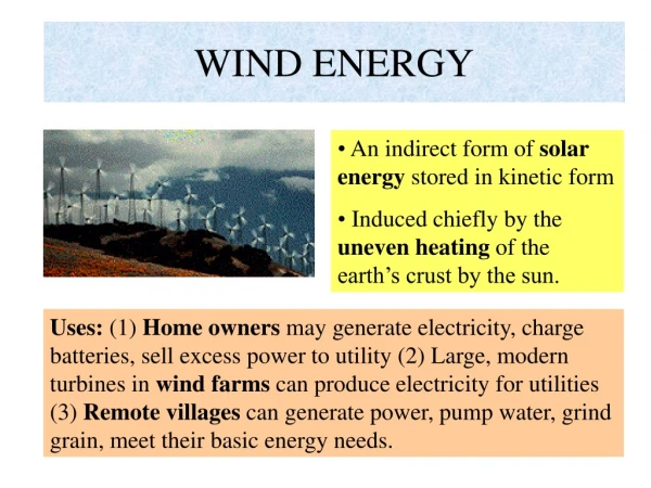
WIND ENERGY • An indirect form of solar energy stored in kinetic form • Induced chiefly by the uneven heating of the earth’s crust by the sun. Uses: (1) Home owners may generate electricity, charge batteries, sell excess power to utility (2) Large, modern turbines in wind farms can produce electricity for utilities (3) Remote villages can generate power, pump water, grind grain, meet their basic energy needs.
Wind Energy, Its Uses and History • Global Wind Resource Potential • Basic Principles of Operation & Components • Power Output and Maximum Efficiency • Types of Wind Mills and Examples • Cost of Wind Power (Capital, O&M, Levelized) • Applicability, Advantages, Disadvantages • Environmental Impact & Risks Topics - Wind Energy
Global Wind Resource • Wind is the movement of air in response to pressure differences within the atmosphere, caused primarily by uneven heating by the sun on the surface of the earth, exerting a force which causes air masses to move from a region of high pressure to a low one. • About 1.7 million TWh of energy each year is generated in the form of wind over the earth’s land masses, much more over the globe as a whole. Only a small fraction can be harnessed to generate useful energy because of competing land use. • A 1991 estimate puts the realizable global wind power potential at 53,000 TWh per year.
National Wind Resources US, UK and China have vast wind resource potential. With only 6% of total land area available for wind, US could generat about 500,000 MW. Present US capacity is 2,500 MW. Philippine capacity stood at 10 kW (Pagudpud) and 120 MW is being planned for Ilocos Norte by PNOC.
Philippine Wind Energy • Philippines has vast potential for wind energy development. Wind Mapping Project of PCIERD-DOST, DOE and NREL estimated the country's potential for wind power at about 76,600 MW. • Ilocos Norte was estimated to have a combined potential of 80 MW. Northern Luzon most attractive with average annual wind of 5.39 m/s. • 10-kW wind turbine generator of PCIED has been supplying the power needs of 23 households in a small fishing village in Pagudpud, Ilocos Norte. • PNOC-EDC is establishing a 120-MW Wind Power Project in Ilocos Norte in 3 phases of 40 MW each.
THE PHILIPPINES HAS A WND POTENTIAL OF 70,000 MW of WIND POWER • Maxum wind power = 300 W/m2 • Turbine size = 500 kW • Hu height = 40 m • Rotor diameter = 38 m • Side to side spacing = 190 m • Front to back spacing = 380 m • Swept area = 1134 m2 • Turbines per sqm = 139 • Capacity per sqm = 6.9 MWkm2
Basic Principles and Components of a Modern Wind Turbine • Turbine rotor captures the wind energy and converts it into mechanical energy fed via a gearbox to a generator • Gearbox / generator housed in an enclosed nacelle with the turbine rotor is attached to its front • Combined rotor and nacelle mounted on a tower fitted with a yawing system keeps the turbine rotor facing into the wind always
Total Power Output of Wind Turbines Total power output of a wind turbine is proportional to the incoming wind velocity raised to the 3rd power: Ptot = m KE = m Vi2 / (2 gc) Watt = J/s = (1 / 2 gc) ρ A Vi3 where m = mass flow = ρ A Vi kg/s ρ = density kg/m3 A = cross-sectional area m2 Vi = incoming velocity m/s gc = conversion factor = 1.0 kg/(N s2)
Ideal or Maximum Theoretical Efficiency of Wind Turbines Maximum power is obtained by differentiating turbine power equation P with respect to exit velocity Ve and equating to zero: P = (1 / 4 gc) ρ A (Vi + Ve) (Vi2 – Ve2) Watt = J/s Solving for optimum exit velocity Ve yields: Ve,opt = (1/3) Vi m/s Pmax = (8 / 27 gc) ρ A Vi3 Watt = J/s Ideal efficiency therefore that could not be more than 60%: EFFmax = Pmax / Ptot = (8/27) / (1/2) = 0.5926
Types of Modern Wind Turbines • Vertical-Axis Windmills – early machines known as Persian windmills; evolved from ship sails made of canvas or wood attached to a large horizontal wheel; when used to grind grain into flour, they were called windmills. • Horizontal-Axis Windmills –first designs had sails built on a post that could face into any wind direction, and were called post mills; evolved throughout the Middle Ages and was used for grinding grain, drainage, pumping, saw-milling.
Examples of Wind Turbines Shown below are examples of a horizontal-axis and vertical-axis wind turbines. Australia California, USA
Cost of Wind Power • Cost of wind power (EIA, 1996): Resource type Intermittent, predictable Capacity factor 20 – 44 % Real levelized cost (1998$) 4 – 6 cents / kWh Construction lead time 1 – 3 years Overnight capital cost $857 / kW Fixed O&M costs $0.256 / kW / year Variable O&M, $/kWh nil • Availability factor of 90% and load factor of 30-40%, sometimes higher at 45% during favorable wind patterns; because of this 1/3 average load factor, a wind farm would be 2.5 times as large as a conventional power plant of same rating and 80% load factor. • Cost of generating wind power in US (EPRI) - $0.05/kWh • Competitive tender bids in UK – as low as $0.032/kWh
Cost of Philippine Wind Power Proposed 120 MW wind farm in Pagudpud, Ilocos: • 1st phase of 40 MW will cost $54 million for 56 units of 750-kW wind turbine generators and 43.5 km transmission system • Selling price to electric coop would be P2.50/kWh below the NPC grid price of P3.00/kWh • 2nd and 3rd phases will cost lower at $36 and $30 million, respectively, for each 40 MW.
Applicability of Wind Power • Economics of wind power depend strongly on wind speed raised to the 3rd power; double the wind speed and energy increases 8 times; actual wind turbines, however, do not yield that much extra power • Wind speed also varies with height ; the higher the turbine is raised above the ground, the better wind regime it will find; a 50m tower can capture 20% more energy than 30m: Vi = Vo (Hi / Ho)α • Economic cut-off wind speed - 6.5m/s at 25m above ground and 7.0m/s at 45m above ground level • Wind speed-height equation makes higher sites more attractive, such as hilly and mountainous sites • Offshore wind speeds are higher and smoother over surface water than land areas, making offshore wind attractive
Advantages of Wind Power • Home owners (250W-25kW) - generate their own electricity, charge batteries, and in some cases, sell excess electricity to the utility, a practice called “net metering” • Hybrid systems – used with other technologies like photovoltaic panels, batteries and diesel generators for round-the-clock renewable power and reliable back-up power; cost-effective at remote, cold sites • Remote villages ( < 100kW) - wind turbines can power small grids, charge batteries, grind grain or pump water, thus improving their quality of life • Wind farms ( > 200kW) - large wind turbines can operate together to produce green power - clean and renewable electricity for utilities; income to rural farmers - $55/acre • Distributed generation – building power plants where power is needed and feeding into distribution rather than transmission systems helps improve the network
Disadvantages of Wind Power • Not steady or reliable - its production does not coincide with demand, hence, it may have to be stored in batteries during off-peak hours or have to be hybrid with other reliable back-up power like diesel generators. • Higher capital and O&M costs - although the cost of wind energy from wind has dropped by 85% over the last 20 years, the need to hybrid wind turbines with other technologies to make it a reliable and stable system tend to increase its capital and operating costs • Some doubts on structural integrity to protect investment - tropical climate of the Philippines which is regularly visited by typhoons with speeds over 100-300 kph, may affect structural integrity of the system even at “stowed position” to withstand such sustained winds over a few hours and sudden wind gusts
Environmental Impact • Green power technology - because wind has only minor impacts on the environment and produces no air pollutants or greenhouse gases - fightsglobal warming • A 1 MW wind farm in UK will prevent the production of 2,200 mt of CO2, 30 mt of SO2 and 10 mt of NOX each year based on UK’s generation mix in 1990. • Aesthetics and visual impacts – elements that influence visual impacts include the spacing, design and uniformity of the turbines. • Birds and other living resources – likely to be affected by the wind turbines as they fly their migration routes. • Noise – wind turbines produce some low level frequency noise when they operate. • TV/radio interference – older turbines with metal blades caused interference; modern composites have reduced this
Risks • Risk associated with the reliability of the wind power resource – should be minimal if an adequate feasibility study has been performed on the site, otherwise, the wind will not blow as it was expected; while the strength of the wind on a particular day and site could not be predicted, wind is normally reliable over longer periods – a windy site will not turn into a windless site. • Risk attached to the use of wind power equipment – while the industry is now well established and many design features have been proven, development is continuous and that always carries a certain risk; wind turbines are becoming larger while experience with them is limited; it is vital to obtain historical performance data to establish its reliability for commercial operations
Wind Resource Estimation and Financial Modeling • Sample wind power curve (individual turbines) • Combined wind power curve table (vertical lookup) – from University of Idano • Wind Mast monitoring (time, speed direction or azimuth) • Converting wind speed (from meters/second to miles per hour) to estimate wind turbine power output • Project Finance Modeling • How to run the project finance models • Monte Carlo Simulation (add-in Excel program)
Sample Wind Turbine Power Curves • GE Wind Turbine Models • Press F9 to recalculate • pc_ge_wind (GE) • Suzlon Wind Turbine Models • Press F9 to recalculate • pc_suzlon (Suzlon)
Combined Power Curve Models • Has 66 OEM with turbine power curves • Wind Power Curves (66 wind turbine models + user defined)2 • Select turbine model number (1-66) • The model uses vertical look-up function of Excel to load the specific data of the wind turbine model • Use wind speed from wind velocity profile of US NREL or 3-Tier (synthesized data) • Use wind mast monitoring (measured data) • Convert the synthesized or measured from m/s to mph, and look-up kW output, generate graph
Synthesize Wind Speed Data • Get Monthly Wind Speed data for 12 months (1st, 15th and 30th of the month)
Steps in creating the table • Read off the 3-TIER chart the readings (average, positive and negative deviations) from the 14th or 15th (V1) of mid-month and 14h or 15th of next month (V2). (in red) • Calculate the month end (30th or 1st) as the average between the two mid-months: • V(30th or 1st) = (V1 + V2)/2 (in blue) • Where V represents the average, pos and neg deviations. • Jan midpoint (10.7, -2.7, 2.8); Feb midpoint (10.1, -2.5, 2.8) • Jan average = (10.7 + 10.1)/2 = 10.4 (blue) • Jan minus = (-2.7 + -2.5)/2 = -2.6 (blue) • Jan plus = (2.8 + 2.8)/2 = 2.8 (blue) • Complete for the nest of the months Feb, Mar … Dec
Interpolate to get the Daily average, minus and plus (1) • Wind Energy Resource Assessment Tool_3TIER Prediction • These calculations are found in the Wind Resource worksheet (tab). • Transfer the average, minus and plus to the wind resource worksheet to the 1st and 16th and 1st of the next month. • Interpolate the daily average speed from the 1st and 14th midpoint. The day 1 formula which you can propagate till the 15th is • C3+(C18-C3)/(A18-A3)*(A4-A3) rounded to 2 decimals • The formula for day 17 which you can propagate till the 30th is • (C18+(C34-C18)/(A34-A18)*(A19-A18) rounded to 2 decimals
Interpolate to get the Daily average, minus and plus (2) • The plus and minus from the wind speed tab is valid from the 1st to the 30th of the month, but the average speed is valid from the 1st, 16th and 30th, from which you do your daily interpolation for 2nd to 15th, and 17th to 29th. • The next step is to convert the daily average interpolated to hourly variation using the rand() function to represent the randomness of the wind speed from the daily average. For the first day of the month, the formula which you can propagate for the entire month and 24 hours is = average + pos * rand() + neg * rand(): • $C3+$AB3*RAND()+$AC3*RAND() and rounded to 2 decs • This will provide your daily and hourly pulses of wind speed
Interpolate to get the Daily average, minus and plus (3) • The next step is to compute the equivalent mph from the m/s speed (mph = m/s x conversion factor, rounded to 1 decs) ROUND(AA3*2.23693929205,1) • Do a vertical look-up on the appropriate wind turbine curve to get the hourly kW output of the wind turbine model from the digitized mph speed (1 decs). • The formula for the Jan 1 and the first hour of the year that you can propagate for the rest of the hours of the year is: (2 decs) • VLOOKUP('Wind Resource'!D371,'GE900'!$E$21:$F$692,2) • Sum all the 24 hourly random kW output from the random speed = annual kWh generation for the particular turbine model • Annual capacity factor = annual kWh generation / (24 * 365 * kw CAPACITY) = % capacity factor
Wind Energy ResourceWind Energy Resource Assessment Tool_Anemometer Measurement2
Combined Power Curves of 66 Wind Turbines (Univ. of Idaho) • Power Curves for 66 wind turbines • Wind Power Curves (66 wind turbine models + user defined)2 • Sample Usage of wind mast data from Sagada, Philippines • Wind Energy Resource Assessment Tool_Anemometer Measurement2
Project Finance Models from OMT ENERGY ENTERPRISES • On-shore wind Models (conventional, wind storage) • ADV Wind Onshore Model4 (PHP) demo2 • ADV Wind Onshore CAES Model4 (PHP) demo2 • Off-shore wind Models (conventional, wind storage) • ADV Wind Offshore Model4 (PHP) demo2 • ADV Wind Offshore CAES Model4 (PHP) demo2
How to Run the Models • Deterministic Model (fixed inputs) • Sensitivity Model (changing inputs – one variable change, set variable changes or scenario) • Stochastic or Probabilistic Model (random inputs) – Monte Carlo Simulation
Deterministic Model (fixed inputs) • Use the deterministic model to determine project feasibility, e.g. given first year tariff, determine the equity and project returns (NPV, IRR, PAYBACK), or given the equity or project target returns, determine the first year tariff. • After changing the blue font inputs, the brown font targets and the red flags, you are now ready to run the deterministic model by using the flowing macros: • The deterministic model has 4 macros (Macro 2 ctrl + f, Macro 4 ctrl + g, Macro 1 ctrl + e, and Macro 3 ctrl + d) for automating your model run: • ADV Wind Onshore Model4 (PHP) demo2
Deterministic Model4 Macros (1, 2, 3, 4) • Macro 2 ctrl + f is used to calibrate the model to meet a given net capacity factor (34.00%), all-in capital cost (2,213 $/kW), fixed O&M (39.55 $/kW/year with the fixed G&A cost initially set to zero), and variable O&M (2.00 $/MWh) which excludes fuel and lubes. Once you have calibrated the fixed O&M, then you may restore the fixed G&A value (say 100 k$/year of general & admin costs for fixed salaries, insurance, security and regulatory costs). You need to do this since the fixed O&M cost target does not include G&A cost. The variable O&M cost target does not include fuel and lube oil costs.
Deterministic Model4 Macros (1, 2, 3, 4) • Macro 4 ctrl + g is used to calibrate the model to meet a given all-in capital cost only (2,213 $/kW) if you are just adjusting the all-in capital cost; otherwise, no need to run if you have run the Macro 2 ctrl + f, and you may proceed to Macro 1 ctrl + e to calculate first year tariff. • Macro 1 ctrl + e is used to set the equity NPV to zero by varying the first year tariff (or feed-in-tariff - FIT). • Macro 3 ctrl + d is used to set the project NPV to zero by varying the first year tariff.
Sensitivity Model (macro 1, 2, 3, 4 and 8) • Use the Sensitivity Model to determine the sequential impact of changing one independent variable (debt ratio, forward exchange rate, unit capacity, plant availability factor, plant degradation rate, fuel GHV, plant GHR, fuel cost, construction period and operating period) at a time on the dependent variables (net capacity factor, equity and project returns such as IRR, NPV, PAYBACK, WACC pre-tax and WACC after-tax, SRMC, and LRMC). In addition to Macro 1, 2, 3 and 4, a new Macro 8 has been added.
Sensitivity Model (macro 1, 2, 3, 4 and 8) • Macro 8 ctrl + q is used to vary scenario or a set of independent variable inputs (Case 1 to 5) using the CHOOSE function of Excel and vary independent variables (debt ratio, exchange rate, unit capacity, availability factor, plant degradation rate, fuel GHV, plant GHR, fuel cost, construction period months, operating period years) one at a time using the TABLES function of Excel to see impact on dependent variables such as equity and project returns (IRR, NPV, PAYBACK), WACC (pre-tax, after-tax), short run marginal cost (SRMC) and long run marginal cost (LRMC) or levelized cost of energy (LCOE).
Running the Stochastic Model (random inputs) • Use the stochastic model to determine project risks during the project development stage. By varying the estimation error on the independent variable (+10% and -10%) and conducting 500-1000 random trials this model will show the upper limit of the estimation error so that the dependent variables will converge to a real value (no error). • Before you can run the MCS model, you have to load and run first the Monte Carlo Simulation add-in program: • MonteCarlito_v1_10 • ADV Wind Onshore Model4 (PHP) MCS demo2 • The stochastic model has 5 macros: (2, 4, 5, 6, 7)
Running the Stochastic Model 5 Macros (2, 4, 5, 6, 7) • Macro 5 - ctrl + m to run the Monte Carlo Simulation (MCS) • If the number of trials is entered as bold font, a distribution graph is generated as a tab for each dependent variable modeled (e.g. equity returns such as NPV, IRR and PAYBACK). The Monte Carlo Simulation add-in calculates the mean, standard error, median, standard deviation, Variance, Skewness, Kurtosis, Expected value (also the mean), Standard deviation * 1.96 and maximum and minimum outcomes at 95% confidence level.
What is being randomized X (random) = X(fixed) * [ 90% + (110% - 90%) * rand() ] Where X = electricity first year tariff, availability factor, debt ration, unit plant capacity, variable and fixed O&M and G&A (OPEX) and capital cost (CAPEX).
Stochastic Variables reported • If the number of trials is entered as bold font, a distribution graph is generated as a tab for each dependent variable modeled (e.g. equity returns such as NPV, IRR and PAYBACK). The Monte Carlo Simulation add-in calculates the mean, standard error, median, standard deviation, Variance, Skewness, Kurtosis, Expected value (also the mean), Standard deviation * 1.96 and maximum and minimum outcomes at 95% confidence level.
THANK YOU Prepared by: Marcial T. Ocampo Energy & Power Consultant mars_ocampo@yahoo.com 63-915-6067949 (GLOBE mobile) OMT ENERGY ENTERPRISES