Download
1 / 39
390 likes | 639 Views
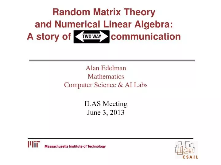
Random Matrix Theory and Numerical Linear Algebra: A story of communication. Alan Edelman Mathematics Computer Science & AI Labs. ILAS Meeting June 3, 2013. An Intriguing Thesis. The results/methodologies from NUMERICAL LINEAR ALGEBRA

E N D
Random Matrix Theoryand Numerical Linear Algebra:A story of communication Alan Edelman Mathematics Computer Science & AI Labs ILAS Meeting June 3, 2013
An Intriguing Thesis The results/methodologies from NUMERICAL LINEAR ALGEBRA would be valuable even if computers had not been built. … but I’m glad we have computers …& I’m especially grateful for the Julia computing system
Eigenvalues of GOE (β=1 means reals) • Naïve Way in four languages: A=randn(n); S=(A+A’)/sqrt(2*n);eig(S) A=randn(n,n);S=(A+A’)/sqrt(2*n);eigvals(S) A=matrix(rnorm(n*n),ncol=n);S=(a+t(a))/sqrt(2*n); eigen(S,symmetric=T,only.values=T)$values; A=RandomArray[NormalDistribution[],{n,n}]; S=(A+Transpose[A])/Sqrt[2*n];Eigenvalues[s]
Eigenvalues of GOE (β=1 means reals) If for you: simulation is just intuition, a check, a figure, or a student project, then software like this is written quickly and victory is declared. • Naïve Way in four languages: A=randn(n); S=(A+A’)/sqrt(2*n);eig(S) A=randn(n,n);S=(A+A’)/sqrt(2*n);eigvals(S) A=matrix(rnorm(n*n),ncol=n);S=(a+t(a))/sqrt(2*n); eigen(S,symmetric=T,only.values=T)$values; A=RandomArray[NormalDistribution[],{n,n}]; S=(A+Transpose[A])/Sqrt[n];Eigenvalues[s]
Eigenvalues of GOE (β=1 means reals) Numerical Linear Algebra For me: Simulation is a chance to research efficiency, Numerical Linear Algebra Style, and this research cycles back to the mathematics! Ψ= • Naïve Way in four languages: A=randn(n); S=(A+A’)/sqrt(2*n);eig(S) A=randn(n,n);S=(A+A’)/sqrt(2*n);eigvals(S) A=matrix(rnorm(n*n),ncol=n);S=(a+t(a))/sqrt(2*n); eigen(S,symmetric=T,only.values=T)$values; A=RandomArray[NormalDistribution[],{n,n}]; S=(A+Transpose[A])/Sqrt[n];Eigenvalues[s]
Tridiagonal Model More Efficient(β=1: Same eigenvalue distribution!) n gi~N(0,2) Julia: eig(SymTridiagonal(d,e)) Storage: O(n) (vs O(n2)) Time: O(n2) (vs O(n3)) (Silverstein, Trotter, general β Dumitriu&E.etc)
Histogram without Histogramming:Sturm Sequences Mentioned in Dumitriu and E 2006, Used theoretically in Albrecht, Chan, and E 2008 • Count #eigs < s: Count sign changes in Det( (A-s*I)[1:k,1:k] ) • Count #eigs in [x,x+h]: Take difference in number of sign changes at x+h and x • Speed comparison vs. naïve way
A good computational trick is a good theoretical trick! Finite Semi-Circle Laws for Any Beta! Finite Tracy-Widom Laws for Any Beta!
Efficient Tracy Widom Simulation • Naïve Way: • A=randn(n); S=(A+A’)/sqrt(2*n);max(eig(S)) • Better Way: • Only create the 10n1/3 initial segment of the diagonal and off-diagonal as the “Airy” function tells us that the max eig hardly depends on the rest • Lead to the notion of the stochastic operator limit
Google Translate (in my dreams) -1 Lost In Translation: eigs = svd’s squared
The Jacobi Random Matrix Ensemble (Constantine 1963) • Suppose A and B are randn(m1,n) and randn(m2,n) • (iid standard normals) • The eigenvalues of • or in symmetric form • has joint density
The Jacobi Ensemble Geometrically • Take random n-hyperplane in Rm(m>n) (uniformly) • Take reference hyperplane (any dimension) • Orthogonal projection of the unit ball in the random hyperplane onto the reference hyperplane is an ellipsoid • Semi-axes lengths are Jacobi cosines:
The GSVD A: m1 x n B: m2 x n [ ]: m x n A B A B Usual Presentation Underlying Geometry Take hyperplane spanned by [ ] X=span( 1st m1 columns of Im) Y=span(last m2 columns of Im)
GSVD Mathematics (Cosine,Sine) Thus any hyperplane is the span of with U’U=V’V=I and C2+S2=I (diagonal) One can directly verify by taking Jacobians projecting out the W’dW directions that we do not care about and further understand CJ = Page 18
Circular Ensembles (Killip and Nenciu 2004 product of tridiagonal solution) A random complex unitary matrix has eigenvalues distributed on the unit circle with density It is desriable to construct random matrices that we can compute with for general beta:
Numerical linear algebra Ammar, Gragg, Reichel (1991) Hessenberg Unitary Matrices Gj = Recalled in Forrester and Rains (2005) Converts Killip and Nenciu to AmmarGraggReichel format Classical orthogonal polynomials on unit circle! Story relates to CMV matrices Verblunsky Coefficients = Schur Parameters
Implementation Remark: Authors would rightly feel all the mathematical information is in their papers. Still this presenter had some considerable trouble gathering enough of the pieces to produce the ultimate arbiter of understanding the result: a working code! Plea: Random Matrix Theory is so valuable to so many, that a pseudocode or code available is a great technology transfer mechanism. Needed facts AmmarGraggReichel format Generating the variables requires some thinking |j| ~ sqrt(1-rand()^ ((2/β)/j)) j = |j|*exp(2*pi*i*rand())
So far: I tried to hint about βIntroduction to Ghosts • G1 is a standard normal N(0,1) • G2 is a complex normal (G1 +iG1) • G4 is a quaternion normal (G1 +iG1+jG1+kG1) • Gβ(β>0) seems to often work just fine “Ghost Gaussian”
Chi-squared 2 Defn: χβ is the sum of βiid squares of standard normals if β=1,2,… Generalizes for non-integer β as the “gamma” function interpolates factorial χ βis the sqrt of the sum of squares (which generalizes) (wikipedia chi-distriubtion) |G1| is χ1 , |G2| is χ2, |G4| is χ4 So why not |Gβ| is χ β? I call χ βthe shadow of Gβ
Real quantity Working with Ghosts
Singular Values of a Ghost Gaussian by a real diagonal (Dubbs, E, Koev, Venkataramana 2013) (see related work by Forrester 2011)
Julia: Parallel Histogram 3rd eigenvalue, pylab plot, 8 seconds!75 processors
Linear Algebra too limited in Lets me put together what I need: e.g.:TridiagonalEigensolver Fast rank one update Arrow matrix eigensolver can surgically use LAPACK without tears
Weekend Julia Run • Histogram of smallest singular value of randn(200) • spiked by doubling the first column • Julia: A=randn(200,200); A(:,1)*=2; • Reduced mathematically to bidiagonal form • Used julia’sbidiagonalsvd • Ran 2.25 billion trials in 20 hours on 75 processors • Naïve serial algorithm would take 16 years
Weekend Julia Run I knew the limiting histogram from my thesis, universality, etc. With this kind of power, I could obtain the first order correction for finite n! Semilogy plot of abs correction and a prediction: This is like having an electron microscope to see small details that would be invisible with conventional tools! • Histogram of smallest singular value of randn(200) • spiked by doubling the first column • Julia: A=randn(200,200); A(:,1)*=2; • Reduced mathematically to bidiagonal form • Used julia’sbidiagonalsvd • Ran 2.25 billion trials in 20 hours on 75 processors • Naïve serial algorithm would take 16 years
Conclusion If you already held Numerical Linear Algebra with high esteem, thanks to random matrix theory, now there are even more reasons! Try julia. (Google: julia)