3-D Bracket
Workshop 10A Loading and Solution. 3-D Bracket. 10A. Loading and Solution 3-D Bracket. Description

3-D Bracket
E N D
Presentation Transcript
Workshop 10A Loading and Solution 3-D Bracket
10A. Loading and Solution3-D Bracket Description • Apply loads to the 3-D bracket model below and solve using the Sparse iterative solver. The model has already been meshed with SOLID95 20-noded bricks, and Young’s Modulus has been set to 30e6 psi. February 7, 2006 Inventory #002269 W10-2
10A. Loading and Solution3-D Bracket Loads and Boundary Conditions Fix kp 28 in z-direction 1000 psi on top area Symmetry B.C. on hole surface February 7, 2006 Inventory #002269 W10-3
10A. Loading and Solution3-D Bracket 1. Enter ANSYS in the working directory specified by your instructor using “bracket-3d” as the jobname. 2. Resume the “bracket-3d.db1” database file: • Utility Menu > File > Resume from … • Select the “bracket-3d.db1” database file, then [OK] • Or issue: RESUME,bracket-3d,db1 3. Enter the solution processor and restrain translations normal to hole surfaces: • Main Menu > Solution > Define Loads > Apply > Structural > Displacement > Symmetry B.C. > On Areas • Pick the areas on the hole surfaces (area numbers 3, 4, 5, and 6), then [OK] • Or issue: /SOLU DA,3,SYMM DA,4,SYMM DA,5,SYMM DA,6,SYMM February 7, 2006 Inventory #002269 W10-4
10A. Loading and Solution3-D Bracket 4. To prevent rigid body motion along the Z axis, constrain UZ translation on keypoint 28: • Main Menu > Solution > Define Loads > Apply > Structural > Displacement > On Keypoints • Enter keypoint number “28” in the ANSYS picking menu followed by [Enter] • [OK] • Set Lab2 = “UZ”, then [OK] • Or issue: DK,28,UZ 5. Apply 1000 psi pressure load to the top surface area of the 3-D bracket: • Main Menu > Solution > Define Loads > Apply > Structural > Pressure > On Areas • Pick the top surface area (area number 11) , then [OK] • Set VALUE = 1000, then [OK] • Or issue: SFA,11,1,PRES,1000 6. Select the Sparse direct solver: • Main Menu > Solution > Analysis Type > Sol’n Controls • Pick the “Sol’n Options” tab • Select the “Sparse direct” solver, then [OK] • Or issue: EQSLV,SPARSE February 7, 2006 Inventory #002269 W10-5
10A. Loading and Solution3-D Bracket 7. Save the database and obtain the solution: • Pick the “SAVE_DB” button in the Toolbar (or select: Utility Menu > File > Save as Jobname.db) • Main Menu > Solution > Solve > Current LS • [OK] • Or issue: SAVE SOLVE 8. After the solution is completed, enter the general postprocessor and plot the von Mises stress (SEQV): • Main Menu > General Postproc > Plot Results > Contour Plot > Nodal Solu • Select Nodal Solution > Stress > von Mises stress, then [OK] • Or issue: /POST1 PLNSOL,S,EQV February 7, 2006 Inventory #002269 W10-6
10A. Loading and Solution3-D Bracket February 7, 2006 Inventory #002269 W10-7
10A. Loading and Solution3-D Bracket 9. Change the viewing angle and replot: • Utility Menu > PlotCtrls > View Settings > Viewing Direction ... • XV = -0.5 • YV = -0.25 • ZV = 1 • [OK] • Or issue: /VIEW,1,-0.5, -0.25, 1 /REPLOT 10. Save the ANSYS database: • Pick the “SAVE_DB” button in the Toolbar February 7, 2006 Inventory #002269 W10-8
Workshop 10BLoading and Solution Connecting Rod
10B. Loading and SolutionConnecting Rod Description • Apply loads to the connecting rod (half-symmetry) model below and solve using the SPARSE solver. The model has already been meshed with SOLID95 20-noded bricks, and Young’s Modulus has been set to 30e6 psi. February 7, 2006 Inventory #002269 W10-10
Constrain UZ DOF on Node 1000 psi on Area Symmetry B.C. on Areas 10B. Loading and SolutionConnecting Rod Loads and Boundary Conditions February 7, 2006 Inventory #002269 W10-11
10B. Loading and SolutionConnecting Rod 1. Enter ANSYS in the working directory specified by your instructor using “conn-rod” as the jobname. 2. Resume the “conn-rod.db1” database file: • Utility Menu > File > Resume from … • Select the “conn-rod.db1” database file, then [OK] • Or issue: RESUME,conn-rod,db1 3. Enter the solution processor and restrain translations normal to the larger hole surfaces: • Main Menu > Solution > Define Loads > Apply > Structural > Displacement > Symmetry B.C. > On Areas • Pick the areas on the hole surfaces (area numbers 8 and 9), then [OK] • Or issue: /SOLU DA,8,SYMM DA,9,SYMM February 7, 2006 Inventory #002269 W10-12
10B. Loading and SolutionConnecting Rod 4. Apply symmetry boundary constraints on all area surfaces at Y=0: • Main Menu > Solution > Define Loads > Apply > Structural > Displacement > Symmetry B.C. > On Areas • Pick the areas on the plane Y=0 (area numbers 7, 10 and 13), then [OK] • Or issue: DA,7,SYMM DA,10,SYMM DA,13,SYMM 5. To prevent rigid body motion along the Z axis, constrain UZ translation on node 702: • Main Menu > Solution > Define Loads > Apply > Structural > Displacement > On Nodes • Enter node number “702” in the ANSYS picking menu followed by [Enter] • [OK] • Set Lab2 = “UZ”, then [OK] • Or issue: D,702,UZ February 7, 2006 Inventory #002269 W10-13
10B. Loading and SolutionConnecting Rod 6. Apply 1000 psi pressure load to area number 11 located on the smaller hole: • Main Menu > Solution > Define Loads > Apply > Structural > Pressure > On Areas • Pick area number 11, then [OK] • Set VALUE = 1000, then [OK] • Or issue: SFA,11,1,PRES,1000 7. Select the Sparse direct solver: • Main Menu > Solution > Analysis Type > Sol’n Control • Pick the “Sol’n Options” tab • Select the “Sparse direct” solver, then [OK] • Or issue: EQSLV,SPARSE 8. Save the database and obtain the solution: • Pick the “SAVE_DB” button in the Toolbar (or select: Utility Menu > File > Save as Jobname.db) • Main Menu > Solution > Solve > Current LS • [OK] • Or issue: SAVE SOLVE February 7, 2006 Inventory #002269 W10-14
10B. Loading and SolutionConnecting Rod 9. After the solution is completed, enter the general postprocessor and plot the von Mises stress (SEQV): • Main Menu > General Postproc > Plot Results > Contour Plot > Nodal Solu • Select Nodal Solution > Stress > von Mises stress, then [OK] • Or issue: /POST1 PLNSOL,S,EQV 10. Save the ANSYS database: • Pick the “SAVE_DB” button in the Toolbar February 7, 2006 Inventory #002269 W10-15
10C. Loading and SolutionWheel Description • Apply loads to the wheel model shown in the next slide and solve using the SPARSE solver. • The model has already been meshed with SOLID45 bricks, SOLID95 pyramids, and SOLID92 tets. • Young’s Modulus has been set to 30e6 psi and density has been set to 0.00073 lbf-s2/in4. February 7, 2006 Inventory #002269 W10-18
Angular Velocity of 525 rad/sec Constrain UY DOF on Node 33 Symmetry B.C. on Areas 10C. Loading and SolutionWheel Loads Symmetry B.C. on Areas February 7, 2006 Inventory #002269 W10-19
10C. Loading and SolutionWheel 1. Enter ANSYS in the working directory specified by your instructor using “wheelb-omega” as the jobname. 2. Resume the “wheelb-omega.db1” database file: • Utility Menu > File > Resume from … • Select the “wheelb-omega.db1” database file, then [OK] • Or issue: RESUME,wheelb-omega,db1 3. Select the areas from the area component name “areas_1”: • Utility Menu > Select > Component Manager • Highlight areas_1 and click on the Select Component/Assembly Icon • Utility Menu > Plot > Areas • Or issue: CMSEL,S,AREAS_1 APLOT 4. Apply symmetry boundary conditions on the selected set of areas: • Main Menu > Solution > Define Loads > Apply > Structural > Displacement > Symmetry B.C. > On Areas • [Pick All] • Or issue: /SOLU DA,ALL,SYMM February 7, 2006 Inventory #002269 W10-20
10C. Loading and SolutionWheel 5. Select everything and plot areas: • Utility Menu > Select > Everything … • Utility Menu > Plot > Areas • Or issue: ALLSEL,ALL,ALL APLOT 6. To prevent rigid body motion, constrain UY translation on node 33: • Main Menu > Solution > Define Loads > Apply > Structural > Displacement > On Nodes • Enter node number “33” in the ANSYS picking menu followed by [Enter] • [OK] • Set Lab2 = “UY”, then [OK] • Or issue: D,33,UY 7. Apply rotational velocity of 525 rad/sec about global Y axis: • Main Menu > Solution > Define Loads > Apply > Structural > Inertia > Angular Velocity > Global • Set OMEGY = 525 • [OK] • Or issue: OMEGA,0,525 February 7, 2006 Inventory #002269 W10-21
10C. Loading and SolutionWheel 8. Select the Sparse direct solver: • Main Menu > Solution > Analysis Type > Sol’n Control • Pick the “Sol’n Options” tab • Select the “Sparse direct” solver, then [OK] • Or issue: EQSLV,SPARSE 9. Save the database and obtain the solution: • Pick the “SAVE_DB” button in the Toolbar (or select: Utility Menu > File > Save as Jobname.db) • Main Menu > Solution > Solve > Current LS • [OK] • Or issue: SAVE SOLVE February 7, 2006 Inventory #002269 W10-22
10C. Loading and SolutionWheel 10. After the solution is completed, enter the general postprocessor and plot the von Mises stress (SEQV): • Main Menu > General Postproc > Plot Results > Contour Plot > Nodal Solu • Select Nodal Solution > Stress > von Mises stress, then [OK] • Or issue: /POST1 PLNSOL,S,EQV February 7, 2006 Inventory #002269 W10-23
10C. Loading and SolutionWheel 11. Expand the results about the Z-axis of local coordinate system 11 (cylindrical): • Utility Menu > WorkPlane > Change Active CS to > Specified Coord Sys … • KCN = 11 • [OK] • Utility Menu > PlotCtrls > Style > Symmetry Expansion > User-Specified Expansion ... • NREPEAT = 16 • TYPE = “Local Polar” • PATTERN = “Alternate Symm” • DY = 22.5 • [OK] • Or issue: CSYS,11 /EXPAND,16,LPOLAR,HALF,,22.5 /REPLOT February 7, 2006 Inventory #002269 W10-24
10C. Loading and SolutionWheel 12. Turn expansion off: • Utility Menu > PlotCtrls > Style > Symmetry Expansion > No Expansion … • Utility Menu > Plot > Replot • Or issue: /EXPAND /REPLOT 13. Save and exit ANSYS: • Pick the “SAVE_DB” button in the Toolbar • Pick the “QUIT” button in the Toolbar February 7, 2006 Inventory #002269 W10-25