Optimizing Dynamic Aperture in Decay Ring Study at Lancaster with MADX Calculations
This study focuses on optimizing the dynamic aperture in a decay ring at Lancaster using MADX calculations. It covers working points, chromaticity, chromaticity corrections, tracking muons, and determining the dynamic aperture. The research discusses the introduction of sextupoles in arcs to compensate for natural chromaticity and minimize dangerous resonances, ultimately reducing aperture loss. Future work includes continuing decay loss studies via G4Beamline, addressing misalignments and field errors, and introducing RF cavities.


Optimizing Dynamic Aperture in Decay Ring Study at Lancaster with MADX Calculations
E N D
Presentation Transcript
Decay Ring Study m. apollonio 22/04/2009 UKNF09 - Lancaster
MADX calculations- Twiss: working points, chromaticity- chromaticity corrections (sextupoles) • tracking and determination of DA • Few words on Decay Losses 22/04/2009 UKNF09 - Lancaster
Lattice: race track scheme 1- original design from C. Prior 2- MADX format by J. Pasternak 22/04/2009 UKNF09 - Lancaster
match straight 1x 1x 12x 1x 1x 7x 7x cell arc 22/04/2009 UKNF09 - Lancaster
Pm = 25 GeV/c L=1608 m 22/04/2009 UKNF09 - Lancaster
Working Point / Chromaticity • Qx = 8.5229 DQx=-11.2149 • Qy = 8.2127 DQy= -9.9437 Dp/p 22/04/2009 UKNF09 - Lancaster
Chromaticity Correction: sextupoles in the arcs 0.5 m 0.4 m 2m 0.5 m 0.7 m 0.7 m Dp/p 22/04/2009 UKNF09 - Lancaster
idea: correcting for nat. chromaticity and avoid dangerous resonances introduces non-linearity reducing DA (see later) Dp/p 22/04/2009 UKNF09 - Lancaster Dp/p 22/04/2009 UKNF09 - Lancaster
Close Up plot for the Working Point 22/04/2009 UKNF09 - Lancaster 22/04/2009 UKNF09 - Lancaster
Dynamic Aperture: MADX+makethin • Tracking muons for 500 turns from P0: • Monitor after N passes [P0,P1,P2,…] • MAX aperture of the ring, Rmax=1m • If Rm > Rmax particle lost • Initial parameters: x=[xm,XM], x’=0, y=y0,y’=0 P1 P0 22/04/2009 UKNF09 - Lancaster
Poincare’ plot (x,x’) with increasing initial X 20000 turns Position – 0
20000 turns Position – 3
Y An example of tracking in a RING with no sextupoles scan x fix y0 X X’ Y’ 500 m transmitted X Y
Y An example of tracking in a RING with correcting sextupoles scan x fix y0 X X’ Y’ 500 m transmitted Y X
baseline acceptance eN=30 mm rad e = eN * mm/P0 bx= 14 m by= 5 m sX= 40 mm sY= 25 mm no-sext: P=27 GeV/c no-sext: P=24 GeV/c no-sext: P=25 GeV/c no-sext: P=26 GeV/c sext-correct: P=26 GeV/c sext-correct: P=25 GeV/c sext-correct: P=24 GeV/c 9x eN 22/04/2009 UKNF09 - Lancaster
ANY (mm rad) no-sext: P=25 GeV/c sext-correct: P=25 GeV/c 30 mm rad acceptance ANX (mm rad) 22/04/2009 UKNF09 - Lancaster
G4Beamline reproduction of the Decay Ring muons let decay electrons straight section matching section arc Dipole virtual detector planes QD QF 22/04/2009 UKNF09 - Lancaster
Conclusions … • initial study on the optics for DKrings (racetrack) with • MADX(working point, opt. functions, dispersion…), • introduction of sextupolesin the arcs to compensate for • natural chromaticity, • resonance diagram, • Dynamic Apertureinvestigated (with and w.o. sextupoles). • … and future work • - continuation od Decay Loss studies via G4Beamline • Initial Study with PTC(not shown here) need to be • consolidated (tracking in thick elements), • MisalignmentandField Errorsto be introduced: see • how DA is degraded, • IntroduceRFcavities 22/04/2009 UKNF09 - Lancaster
2ns 3ns Flux Determination • 1021m/yr (1yr = 200 days) = 5.8x10¹³m/s • 50 Hz (proton) rep. rate • 1.15x10¹²m/(train-triplet) 3.8x10¹¹m/train • 3 bunch trains, 440 ns long (88 bunches of 2 ns each) • 3.8x10¹¹m/T(440ns)= 140 mA • 4.4x10⁹ m/B(2ns) = 350 mA • tm=2.2*(E/m) msec = 520 msec 88 B (T) (S) 440ns 1200ns 1640ns (TS) tm=520 msec 2x10⁴msec = 50Hz rep.rate
How to ? Current Transformers with a) Ib=150 mA / 350 mA b) integration time 440ns / 2 ns c) good frequency response (200 MHz) [do we want/need to measure the single bunch?] NB: F(t) ~ e-t/tm , so after 3.7 msec we have 100 mA / train (minimum detectable current?) - which precision do we need? - when do we stop being sensitive? Can we use complementary methods? e.g. counting electron flux from m decays in the straights?
Possible NF-LAYOUT at RAL? IDS meeting - CERN 24