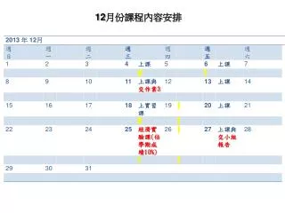
12 月份課程內容安排
470 likes | 650 Views
12 月份課程內容安排. 演講加分機會. R. GLENN HUBBARD. ANTHONY PATRICK O’BRIEN. Economics FOURTH EDITION. 11. Technology, Production, and Costs. CHAPTER. Chapter Outline and Learning Objectives. 低成本航空公司 [ 資料 來源:維基百 科 ]

12 月份課程內容安排
E N D
Presentation Transcript
R. GLENNHUBBARD ANTHONY PATRICKO’BRIEN Economics FOURTH EDITION
11 Technology, Production, and Costs CHAPTER Chapter Outline and Learning Objectives
低成本航空公司 [資料來源:維基百科] • 航空業競爭激烈,中小型航空公司常以低廉的票價取勝。美國由於幅員遼闊,飛機是經常使用的交通工具,許多旅客只希望能夠快速安全地到達目的地,並不需要很高級的服務。 • 營運方式 • 降低成本通常有下列幾種方式。 • 降低營業成本 • 飛行路線以中短程為主,多為鄰近地區。 • 機隊單一化;部份航空公司使用二手飛機營運。 • 減少使用大型機場。 • 減少租用機場內較昂貴的設施,比如登機橋。 • 減少空勤及地勤員工的薪說水,有些改以約聘方式僱用。
簡化機內服務 • 簡化機艙內的清掃,並減少飛機停留時間。 • 減少公共活動區域,增加班機座位。 • 機內飲食簡化,甚至改成付費制。 • 積極販售機內商品或食物,以增加運費以外的收入。 • 不提供或只提供收費及有限的機上視聽娛樂器材、雜誌及報紙。 • 行李托運的免費重量降低,甚至需要額外付費。 • 降低票務成本 • 客艙等級單一化。 • 積極推廣網路訂票及網上辦理登記手續,不提供選位服務,改以自由入座。 • 依飛行時段訂定不同票價。 • 愈早訂票票價愈低。 • 點對點的營運方式並減少轉機的服務。 • 不使用傳統硬紙板式帶磁條的登機證,改用包含條碼的普通紙質登機證。 • 部份低成本航空沒有退款服務。如果臨時更改時間及地點,會額外索取手續費,有時手續費超過當初購買的費用。
前進美國 鴻海賓州投資12億 [資料來源:工商時報2013/11/23] • 響應美國「Advanced Manufacturing in America」政策,規畫在美國賓州投資4,000萬美元,從事研發、自動化與擴產,作為進軍美國高階精密製造、潛力項目投資的行動第一步。 • 計劃和卡內基美隆大學展開製造研發計畫,借重該大學在全球機器人學的優勢,預計2年內投資1,000萬美元,專注在機器人自動化科技研發合作。 • 2年內實際投資富士康美東公司3,000萬美元,目前規畫新聘500名員工,擴大原本研發小組的編制,而成為完善的高階製造業生產鏈。 • 郭台銘強調,來美投資並非外界所推測為特定品牌的產品製造,而是在美國打造高難度、高技術、高附加價值的製造業,並針對未來科技趨勢包括八屏電子產品,就近在美國利用自動化和機器人進行生產,讓製造與運送成本大幅降低
提高品質,降低成本 • [資料來源:經理人Manager Today整理‧撰文 / 吳升皓] • 王永慶自述的成功之道就是:「不斷追求合理化,降低成本,以物美價廉取勝。」認為台塑在石化業中扮演原料供應的角色,所以應該致力於提供下游客戶物美價廉的產品;而當下游客戶獲得經營助力,得以順利推展業務,將有利於雙方締結緊密的合作關係,連帶地促使台塑擴充經營規模。 • 要做到高品質、低價格,最重要的關卡就是成本分析。 • 一般企業做到單位成本,把單位成本分為固定成本及變動成本,將相關項目每月的耗用量及金額做比較,再取平均數或最低數目做為控制目標,並觀察變動、分析變動原因,當發現有可以節省刪減時,再做修改。 • 王永慶認為傳統的分析方式做得不徹底,得出的結論會與實際有所落差,追究原因後發現,問題可能出在負責成本分析的人,並不是實際工作者,導致分析數字不夠精準;也可能是分析的深度不夠,以致於不能發揮控制作用;甚至有可能是因為成本分析後得出的數字過於寬鬆,若再加上獎勵辦法的實施,很容易就會造成績效獎金拿得容易。 • 王永慶提出「單元成本」的概念,亦即由很多、很小的單元,組成一個成本單元,再由成本單元組合出真正的成本。以財務費用為例,台塑會再細分為原料、製造過程、產品或營業上的財務費用。
此外,台塑還從下列三方面著手降低成本。 • 降低建廠成本 • 培養內部機械人才 • 自行設計、製造生產工具。 • 例如台塑的關係企業永嘉公司,在1980年建廠時,只需向國外訂購製程和機 器,建廠成本比一般水準節省了40%。 • 降低生產成本,節省能源支出 • 例如台電在過去曾兩度提高油電價格,共計造成台塑17億能源費用的增加,為此成立能源改善小組,負責督察節約能源執行狀況及提出建議。 • 降低營銷成本 • 建造招待所:配合台塑各級主管至各廠區出差投宿,在台北、林口、宜蘭、彰化、高雄至美國德州都有設置。招待所通常設在廠區,不但省下交通費和住宿費,也縮短了往返廠區與旅館的時間。 • 王永慶降低成本的做法,曾被質疑價格和品質難以兩全,但他的著眼點在於「合理」,因此真正被刪減掉的是過程中非必要的支出。這樣的做法,也讓台塑落實了「節省一塊錢,就等於淨賺一塊錢」的理念,成就了台塑企業經營的利潤,並且兼顧顧客的利益。
Technology: An Economic Definition 11.1 LEARNING OBJECTIVE Define technology and give examples of technological change.
The basic activity of a firm is to use inputs, such as workers, machines, and natural resources, to produce outputs of goods and services. Technology(技術)The processes a firm uses to turn inputs into outputs of goods and services. Technological change (技術改變)A change in the ability of a firm to produce a given level of output with a given quantity of inputs.
The Short Run and the Long Run in Economics 11.2 LEARNING OBJECTIVE Distinguish between the economic short run and the economic long run.
Short run (短期)The period of time during which at least one of a firm’s inputs is fixed. Long run(長期)The period of time in which a firm can vary all its inputs, adopt new technology, and increase or decrease the size of its physical plant. The Difference between Fixed Costs and Variable Costs (固定成本與變動成本的差異) Total cost (總成本)The cost of all the inputs a firm uses in production. Variable costs (變動成本)Costs that change as output changes. Fixed costs (固定成本)Costs that remain constant as output changes. All of a firm’s costs are either fixed or variable, so we can state the following: Total cost = Fixed cost + Variable cost or, using symbols: TC = FC + VC
Implicit Costs (隱藏成本)versus Explicit Costs(外顯成本) Opportunity cost (機會成本)The highest-valued alternative that must be given up to engage in an activity. Explicit cost (外顯成本)A cost that involves spending money. Implicit cost (隱藏成本)A nonmonetary opportunity cost. Economic depreciation is the difference between the amount paid for capital at the beginning of the year and the amount it could be sold for at the end of the year. Explicit costs are sometimes called accounting costs. Economic costs include both accounting costs and implicit costs.
Jill Johnson’s Costs per Year Table 11.1 The entries in red are explicit costs, and the entries in blue are implicit costs.
Production function (生產函數)The relationship between the inputs employed by a firm and the maximum output it can produce with those inputs. Short-Run Production and Cost at Jill Johnson’s Restaurant Table 11.2
A First Look at the Relationship between Production and Cost Figure 11.1a Graphing Total Cost and Average Total Cost at Jill Johnson’s Restaurant We can use the information from Table 11.2 to graph the relationship between the quantity of pizzas Jill produces and her total cost and average total cost. Panel (a) shows that total cost increases as the level of production increases.
Average total cost (平均總成本)Total cost divided by the quantity of output produced. Figure 11.1b Graphing Total Cost and Average Total Cost at Jill Johnson’s Restaurant Here we see that the average total cost is roughly U shaped: As production increases from low levels, average total cost falls before rising at higher levels of production. To understand why average total cost has this shape, we must look more closely at the technology of producing pizzas, as shown by the production function.
The Marginal Product of Labor and the Average Product of Labor 11.3 LEARNING OBJECTIVE Understand the relationship between the marginal product of labor and the average product of labor.
Marginal product of labor (邊際勞動生產力) The additional output a firm produces as a result of hiring one more worker. The Marginal Product of Labor at Jill Johnson’s Restaurant Table 11.3 An increase in the marginal product can result from the division of labor and from specialization. Law of diminishing returns (報酬遞減法則)The principle that, at some point, adding more of a variable input, such as labor, to the same amount of a fixed input, such as capital, will cause the marginal product of the variable input to decline.
Graphing Production Figure 11.2 Total Output and theMarginal Product of Labor In panel (a), output increases as more workers are hired, but the increase in output does not occur at a constant rate. Because of specialization and the division of labor, output at first increases at an increasing rate, with each additional worker hired causing production to increase by a greater amount than did the hiring of the previous worker. After the third worker has been hired, hiring more workers while keeping the number of pizza ovens constant results in diminishing returns. When the point of diminishing returns is reached, production increases at a decreasing rate. Each additional worker hired after the third worker causes production to increase by a smaller amount than did the hiring of the previous worker. In panel (b), the marginal product of labor is the additional output produced as a result of hiring one more worker. The marginal product of labor rises initially because of the effects of specialization and division of labor, and then it falls due to the effects of diminishing returns.
The Relationship between Marginal Product and Average Product邊際產出與平均產出的關係 Average product of labor (平均勞動生產力)The total output produced by a firm divided by the quantity of workers. The average product of labor is the average of the marginal products of labor. Using the numbers from Table 11.3, we can find the average product of labor for three workers:
An Example of Marginal and Average Values: College Grades Figure 11.3 Marginal and Average GPAs The relationship between marginal and average values for a variable can be illustrated using GPAs. We can calculate the GPA Paul earns in a particular semester (his “marginal GPA”), and we can calculate his cumulative GPA for all the semesters he has completed so far (his “average GPA”). Paul’s GPA is only 1.50 in the fall semester of his first year. In each following semester through the fall of his junior year, his GPA for the semester increases—raising his cumulative GPA. In Paul’s junior year, even though his semester GPA declines from fall to spring, his cumulative GPA rises. Only in the fall of his senior year, when his semester GPA drops below his cumulative GPA, does his cumulative GPA decline.
The Relationship between Short-Run Production and Short-Run Cost 11.4 LEARNING OBJECTIVE Explain and illustrate the relationship between marginal cost and average total cost. Marginal cost (邊際成本)The change in a firm’s total cost from producing one more unit of a good or service.
Jill Johnson’s Marginal Cost and Average Total Cost of Producing Pizzas Figure 11.4 We can use the information in the table to calculate Jill’s marginal cost and average total cost of producing pizzas. For the first two workers hired, the marginal product of labor is increasing, which causes the marginal cost of production to fall. For the last four workers hired, the marginal product of labor is falling, which causes the marginal cost of production to increase. So, the marginal cost curve falls and then rises—that is, has a U shape—because the marginal product of labor rises and then falls. As long as marginal cost is below average total cost, average total cost will be falling. When marginal cost is above average total cost, average total cost will be rising. The relationship between marginal cost and average total cost explains why the average total cost curve also has a U shape.
Why Are the Marginal and Average Cost Curves U Shaped?為何邊際與平均成本曲線為U型? When the marginal product of labor is rising, the marginal cost of output is falling. When the marginal product of labor is falling, the marginal cost of production is rising. We can conclude that the marginal cost of production falls and then rises—forming a U shape—because the marginal product of labor rises and then falls.
Graphing Cost Curves 11.5 LEARNING OBJECTIVE Graph average total cost, average variable cost, average fixed cost, and marginal cost.
Average fixed cost (平均固定成本)Fixed cost divided by the quantity of output produced. Average variable cost (平均變動成本)Variable cost divided by the quantity of output produced. With Q being the level of output, we have: Notice that average total cost is the sum of average fixed cost plus average variable cost: ATC = AFC + AVC
Figure 11.5 Costs at Jill Johnson’s Restaurant • Jill’s costs of making pizzas are shown in the table and plotted in the graph. • Notice three important facts about the graph: • The marginal cost (MC), average total cost (ATC), and average variable cost (AVC) curves are all U shaped, and • the marginal cost curve intersects both the average variable cost curve and average total cost curve at their minimum points. • (2) As output increases, average fixed cost (AFC) gets smaller and smaller. • (3) As output increases, the difference between average total cost and average variable cost decreases.
Understand the following three key facts about Figure 11.5: When marginal cost is less than average variable cost or average total cost, it causes them to decrease. When it is greater, it causes them to increase. Therefore, when they are equal, they must be at their minimum points where the marginal cost curve intersects. All three of these curves are U shaped. Average fixed cost gets smaller and smaller as output increases because in calculating average fixed cost, we are dividing something that gets larger and larger—output—into something that remains constant—fixed cost. Firms often refer to this process of lowering average fixed cost by selling more output as “spreading the overhead” (where “overhead” refers to fixed costs). The difference decreases between average total cost and average variable cost because it is representing average fixed cost, which gets smaller as output increases.
Costs in the Long Run 11.6 LEARNING OBJECTIVE Understand how firms use the long-run average cost curve in their planning.
In the long run, all costs are variable. There are no fixed costs in the long run. Economies of Scale (規模經濟) Long-run average cost curve (長期平均成本線)A curve that shows the lowest cost at which a firm is able to produce a given quantity of output in the long run, when no inputs are fixed. Economies of scale The situation when a firm’s long-run average costs fall as it increases the quantity of output it produces.
Figure 11.6 The Relationship between Short-Run Average Cost and Long-Run Average Cost If a small bookstore expects to sell only 1,000 books per month, it will be able to sell that quantity at the lowest average cost of $22 per book. A larger bookstore will be able to sell 20,000 books per month at a lower cost of $18 per book. A bookstore selling 20,000 books per month and a bookstore selling 40,000 books per month will experience constant returns to scale and have the same average cost. The bookstore selling 20,000 books per month will have reached minimum efficient scale. Very large bookstores will experience diseconomies of scale, and their average costs will rise as sales increase beyond 40,000 books per month.
Long-Run Average Total Cost Curves for Bookstores Constant returns to scale (規模報酬不變)The situation in which a firm’s long-run average costs remain unchanged as it increases output. Minimum efficient scale (最小效率規模)The level of output at which all economies of scale are exhausted. Diseconomies of scale (規模不經濟)The situation in which a firm’s long-run average costs rise as the firm increases output.
Don’t Let This Happen to You Don’t Confuse Diminishing Returns with Diseconomies of Scale Diminishing returns applies only to the short run, when at least one of the firm’s inputs, such as the quantity of machinery it uses, is fixed. Diseconomies of scale apply only in the long run, when the firm is free to vary all its inputs, can adopt new technology, and can vary the amount of machinery it uses and the size of its facility. • Your Turn:Test your understanding by doing related problem 6.14 at the end of this chapter. MyEconLab
A Summary of Definitions of Cost Table 11.4
Appendix Using Isoquants and Isocost Lines to Understand Production and Cost LEARNING OBJECTIVE Use isoquants and isocost lines to understand production and cost. Isoquants Firms search for the cost-minimizing combination of inputs that will allow them to produce a given level of output. This combination depends on two factors: 1. Technology—which determines how much output a firm receives from employing a given quantity of inputs. 2. Input prices—which determine the total cost of each combination of inputs. An Isoquant Graph Isoquant(等量曲線)A curve that shows all the combinations of two inputs, such as capital and labor, that will produce the same level of output.
Figure 11A.1 Isoquants Isoquants show all the combinations of two inputs, in this case capital and labor, that will produce the same level of output. For example, the isoquant labeled Q = 5,000 shows all the combinations of ovens and workers that enable Jill to produce that quantity of pizzas per week. At point A, she produces 5,000 pizzas using 3 ovens and 6 workers, and at point B, she produces the same output using 2 ovens and 10 workers. With more ovens and workers, she can move to a higher isoquant. For example, with 4 ovens and 12 workers, she can produce at point C on the isoquantQ = 10,000. With even more ovens and workers, she could move to the isoquantQ = 13,000.
The Slope of an Isoquant Marginal rate of technical substitution (MRTS) (邊際技術替代率)The rate at which a firm is able to substitute one input for another while keeping the level of output constant. The MRTS is equal to the change in capital divided by the change in labor, so it will become smaller (in absolute value) as we move down an isoquant. Isocost Lines A firm wants to produce a given quantity of output at the lowest possible cost. We can show the relationship between the quantity of inputs used and the firm’s total cost by using an isocost line. Isocost line (等成本線)All the combinations of two inputs, such as capital and labor, that have the same total cost.
Graphing the Isocost Line An Isocost Line Figure 11A.2 The isocost line shows the combinations of inputs with a total cost of $6,000. The rental price of ovens is $1,000 per week, so if Jill spends the whole $6,000 on ovens, she can rent 6 ovens (point A). The wage rate is $500 per week, so if Jill spends the whole $6,000 on workers, she can hire 12 workers. As she moves down the isocost line, she gives up renting 1 oven for every 2 workers she hires. Any combinations of inputs along the line or inside the line can be purchased with $6,000. Any combinations that lie outside the line cannot be purchased with $6,000.
The Slope and Position of the Isocost Line The slope of the isocost line is equal to the ratio of the price of the input on the horizontal axis divided by the price of the input on the vertical axis multiplied by -1. Figure 11A.3 The Position of the Isocost Line The position of the isocost line depends on the level of total cost. As total cost increases from $3,000 to $6,000 to $9,000 per week, the isocost line shifts outward. For each isocost line shown, the rental price of ovens is $1,000 per week, and the wage rate is $500 per week.
Choosing the Cost-Minimizing Combination of Capital and Labor Figure 11A.4 Choosing Capital and Labor to Minimize Total Cost Jill wants to produce 5,000 pizzas per week at the lowest total cost. Point B is the lowest-cost combination of inputs shown in the graph, but this combination of 1 oven and 4 workers will produce fewer than the 5,000 pizzas needed. Points C and D are combinations of ovens and workers that will produce 5,000 pizzas, but their total cost is $9,000. The combination of 3 ovens and 6 workers at point A produces 5,000 pizzas at the lowest total cost of $6,000.
Different Input Price Ratios Lead to Different Input Choices Figure 11A.5 Changing Input Prices Affect the Cost-Minimizing Input Choice As the graph shows, the input combination at point A, which was optimal for Jill, is not optimal for a businessperson in China. Using the input combination at point A would cost businesspeople in China more than $6,000. Instead, the Chinese isocost line is tangent to the isoquant at point B, where the input combination is 2 ovens and 10 workers. Because ovens cost more in China but workers cost less, a Chinese firm will use fewer ovens and more workers than a U.S. firm, even if it has the same technology as the U.S. firm.
Another Look at Cost Minimization At the point of cost minimization, the isoquant and isocost lines are tangent, so they have the same slope. Therefore, at the point of cost minimization, the marginal rate of technical substitution (MRTS) is equal to the wage rate divided by the rental price of capital. The slope of the isoquant tells us the rate at which a firm is able to substitute labor for capital, given existing technology. The slope of the isocost line tells us the rate at which a firm is able to substitute labor for capital, given current input prices. Only at the point of cost minimization are these two rates the same. In this chapter, we defined the marginal product of labor (MPL) as the additional output produced by a firm as a result of hiring one more worker. Similarly, we can define the marginal product of capital (MPK) as the additional output produced by a firm as a result of using one more machine.
When Jill uses fewer ovens but more workers, the gain in output from the additional workers is equal to the loss from the smaller quantity of ovens because total output remains the same along an isoquant. Therefore: −Change in the quantity of ovens × MPK = Change in the quantity of workers × MPL If we rearrange terms, we have the following: Because the first expression is the slope of the isoquant, it is equal to the marginal rate of technical substitution (multiplied by negative 1). So, we can write:
The slope of the isocost line equals the wage rate (w) divided by the rental price of capital (r). We saw earlier in this appendix that at the point of cost minimization, the MRTS equals the ratio of the prices of the two inputs. Therefore: We can rewrite this to show that at the point of cost minimization: This last expression tells us that to minimize cost for a given level of output, a firm should hire inputs up to the point where the last dollar spent on each input results in the same increase in output. If this equality did not hold, a firm could lower its costs by using more of one input and less of the other.
Expansion path (擴張路徑)A curve that shows a firm’s cost-minimizing combination of inputs for every level of output. Figure 11A.6 The Expansion Path The tangency points A, B, and C lie along the firm’s expansion path, which is a curve that shows the cost-minimizing combination of inputs for every level of output. In the short run, when the quantity of machines is fixed, the firm can expand output from 75 bookcases per day to 100 bookcases per day at the lowest cost only by moving from point B to point D and increasing the number of workers from 60 to 110. 0 In the long run, when it can increase the quantity of machines it uses, the firm can move from point D to point C,thereby reducing its total costs of producing 100 bookcases per day from $4,250 to $4,000. The expansion path represents the least-cost combination of inputs to produce a given level of output in the long run, when the firm is able to vary the levels of all of its inputs.