Download
1 / 79
1.89k likes | 3.36k Views
Mechanical Behavior of Materials. ME 2105 Dr. R. Lindeke, Ph.D. Chapter 6: Behavior Of Material Under Mechanical Loads = Mechanical Properties. Stress and strain : What are they and why are they used instead of load and deformation Elastic behavior:

E N D
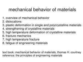
Mechanical Behavior of Materials ME 2105 Dr. R. Lindeke, Ph.D.
Chapter 6: Behavior Of Material Under Mechanical Loads = Mechanical Properties. • Stress and strain: • What are they and why are they used instead of load and deformation • Elastic behavior: • Recoverable Deformation of small magnitude • Plastic behavior: • Permanent deformation We must consider which materials are most resistant to permanent deformation? • Toughness and ductility: • Defining how much energy that a material can take before failure. How do we measure them? • Hardness: • How we measure hardness and its relationship to material strength
• Typical tensile specimen (ASTM A-bar) specimen extensometer gauge length Stress-Strain: Testing Uses Standardized methods developed by ASTM for Tensile Tests it is ASTM E8 • Typical tensile test machine Adapted from Fig. 6.3, Callister 7e. (Fig. 6.3 is taken from H.W. Hayden, W.G. Moffatt, and J. Wulff, The Structure and Properties of Materials, Vol. III, Mechanical Behavior, p. 2, John Wiley and Sons, New York, 1965.)
Comparison of Units: SI and Engineering Common (in US) One other conversion: 1 GPa = 103MPa
The Engineering Stress - Strain curve Divided into 2 regions ELASTIC PLASTIC
Engineering Stress: • Tensile stress, s: • Shear stress, t: F F F t t Area, A F s Area, A F s F t F F t s F t = F lb N t s = A = f or o 2 2 in m A o original area before loading Stress has units: N/m2 (MPa) or lbf/in2 we can also see the symbol ‘s’ used for engineering stress
Common States of Stress F F A = cross sectional o area (when unloaded) F = s s s A o M F s A o A c F s = t A o M 2R • Simple tension: cable Ski lift(photo courtesy P.M. Anderson) • Torsion (a form of shear): drive shaft Note: t = M/AcR here. Where M is the “Moment” Ac shaft area & R shaft radius
• Hooke's Law: F s = Ee s d /2 A o d /2 E L Lo w o e Linear- elastic Linear: Elastic Properties • Modulus of Elasticity, E: (also known as Young's modulus) Units: E: [GPa] or [psi] Here: The Black Outline is Original, Green is after application of load
Typical Example: • Aluminum tensile specimen, square X-Section (16.5 mm on a side) and 150 mm long • Pulled in tension to a load of 66700 N • Experiences elongation of: 0.43 mm • Determine Young’s Modulus if all the deformation is recoverable
Figure 6.2Load-versus-elongation curve obtained in a tensile test. The specimen was aluminum 2024-T81.
Figure 6.3Stress-versus-strain curve obtained by normalizing the data of Figure 6.2 for specimen geometry.
OTHER COMMON STRESS STATES (1) A o Canyon Bridge, Los Alamos, NM (photo courtesy P.M. Anderson) F = s Balanced Rock, Arches A National Park o • Simple compression: Note: compressive structure member (s < 0 here). (photo courtesy P.M. Anderson)
OTHER COMMON STRESS STATES (2) Fish under water s > 0 q s< 0 s > 0 z h • Bi-axial tension: • Hydrostatic compression: Pressurized tank (photo courtesy P.M. Anderson) (photo courtesy P.M. Anderson)
Engineering Strain (resulting from engineering stress): d /2 d L e = e = L L w L o w o o o d /2 L g = Dx/y= tan q • Lateral(Normal to load) strain: • Tensile(parallel to load) strain: - d Here: The Black Outline is Original, Green is after application of load • Shear strain: q Strain is always Dimensionless! x y 90º - q 90º We often see the symbol ‘e’ used for engineering strain
Figure 6.11The Poisson’s ratio (ν) characterizes the contraction perpendicular to the extension caused by a tensile stress. metals: n 0.33ceramics: n 0.25polymers: n 0.40
Other Elastic Properties M t G simple torsion test g M P • Elastic Bulk modulus, K: P P P D V D V P = - K V o V pressure test: Init. vol =Vo. Vol chg. = DV K o • Special relations for isotropic materials: E E = = K G 3(1-2n) 2(1+n) • Elastic Shear modulus, G: t = Gg E is Modulus of Elasticity is Poisson’s Ratio
Figure 6.4 The Yield Strength is defined relative to the intersection of the stress–strain curve with a “0.2% offset.” Yield strength is a convenient indication of the onset of plastic deformation.
Figure 6.10For a low-carbon steel, the stress-versus-strain curve includes both an upper and lower yield point.
Figure 6.5 Elastic recovery occurs when stress is removed from a specimen that has already undergone plastic deformation.
Lets Try an Example Problem GIVENS (load and length as test progresses):
Leads to the Eng. Stress/Strain Curve: T. Str. 1245 MPa F. Str 970 MPa Y. Str. 742 MPa %el 11.5% E 195 GPa (by regression)
Figure 6.7Neck down of a tensile test specimen within its gage length after extension beyond the tensile strength. (Courtesy of R. S. Wortman.)
Figure 6.8True stress (load divided by actual area in the necked-down region) continues to rise to the point of fracture, in contrast to the behavior of engineering stress. (From R. A. Flinn and P. K. Trojan, Engineering Materials and Their Applications, 2nd ed., Houghton Mifflin Company, 1981, used by permission.)
True Stress & Strain Note: Stressed Area changes when sample is deformed (stretched) • True stress • True Strain Adapted from Fig. 6.16, Callister 7e.
Figure 6.25 Forest of dislocations in a stainless steel as seen by a transmission electron microscope [Courtesy of Chuck Echer, Lawrence Berkeley National Laboratory, National Center for Electron Microscopy.]
Returning to our Example – True Properties Necking Began
s s large Strain hardening y 1 s y small Strain hardening 0 e e T Strain Hardening • An increase in sy due to continuing plastic deformation. • Curve fit to the stress-strain response: hardening exponent: ( ) n n = 0.15 (some steels) s = K T n = 0.5 (some coppers) “true” strain: ln(Li /Lo) “true” stress (F/Ai)
We Compute T = KTnto complete our True Stress True Strain plot (plastic data to necking) • Take Logs of both T and T • Regress the values from Yielding to Necking • Gives a value for n (slope of line) and K (its T when T=1) • Plot as a line beyond necking start
Stress Strain Plot w/ True Values n 0.242 K 2617 MPa
TOUGHNESS Is a measure of the ability of a material to absorb energy up to fracture High toughness = High yield strength and ductility Important Factors in determining Toughness: 1. Specimen Geometry & 2. Method of load application Dynamic (high strain rate) loading condition (Impact test) 1. Specimen with notch- Notch toughness 2. Specimen with crack- Fracture toughness Static (low strain rate) loading condition (tensile stress-strain test) 1. Area under stress vs strain curve up to the point of fracture.
Figure 6.9The toughness of an alloy depends on a combination of strength and ductility.
Toughness – Generally considering various materials small toughness (ceramics) E ngineering tensile large toughness (metals) s stress, very small toughness Adapted from Fig. 6.13, Callister 7e. (unreinforced polymers) e Engineering tensile strain, • Energy to break a unit volume of material • Approximate by the area under the stress-strain curve. Brittle fracture: elastic energyDuctile fracture: elastic + plastic energy
Deformation Mechanisms – from Macro-results to Micro-causes Slip Systems • Slip plane - plane allowing easiest slippage • Wide interplanarspacings - highest planar densities • Slip direction- direction of movement - Highest linear densities • FCC Slip occurs on {111} planes (close-packed) in <110> directions (close-packed) => total of 12 slip systems in FCC • in BCC & HCP other slip systems occur Adapted from Fig. 7.6, Callister 7e.
Figure 6.19 Sliding of one plane of atoms past an adjacent one. This high-stress process is necessary to plastically (permanently) deform a perfect crystal.
Applied tensile Relation between Resolved shear s s tR stress: = F/A and tR stress: = F /A s s F tR slip plane normal, ns FS /AS = A l f F cos A / cos tR f nS F AS slip direction l A FS FS AS slip direction F slip direction tR Stress and Dislocation Motion • Crystals slip due to a resolved shear stress, tR. • Applied tension can produce such a stress. Note: By definition is the angle between the stress direction and Slip direction; is the angle between the normal to slip plane and stress direction
Critical Resolved Shear Stress typically 10-4GPa to 10-2 GPa s s s tR s = 0 tR /2 = 0 tR = f l =90° l =90° =45° f =45° • Condition for dislocation motion: • Crystal orientation can make it easy or hard to move dislocation
Generally: Resolved (shear stress) is maximum at = = 45 And CRSS = y/2 for dislocations to move (in single crystals)
Determining and angles for Slip in Crystals(single X-tals this is easy!) • and angles are respectively angle between tensile direction and Normal to Slip plane and angle between tensile direction and slip direction (these slip directions are material dependent) • In General for cubic xtals, angles between directions are given by: • Thus for metals we compare Slip System (normal to slip plane is a direction with exact indices as plane) to applied tensile direction using this equation to determine the values of and to plug into the R equation to determine if slip is expected As we saw earlier!
Slip Motion in Polycrystals s 300 mm • Stronger since grain boundaries pin deformations • Slip planes & directions (l, f) change from one crystal to another. • tRwill vary from one crystal to another. • The crystal with the largest tR yields first. • Other (less favorably oriented) crystals yield (slip) later. (courtesy of C. Brady, National Bureau of Standards [now the National Institute of Standards and Technology, Gaithersburg, MD].)
After seeing the effect of poly crystalline materials we can say (as related to strength): • Ordinarily ductility is sacrificed when an alloy is strengthened. • The relationship between dislocation motion and mechanical behavior of metals is significance to the understanding of strengthening mechanisms. • The ability of a metal to plastically deform depends on the ability of dislocations to move. • Virtually all strengthening techniques rely on this simple principle: Restricting or Hindering dislocation motion renders a material harder and stronger. • We will consider strengthening single phase metals by: grain size reduction, solid-solution alloying, and strain hardening
apply known force measure size e.g., of indentation after Hardened 10 mm sphere removing load Smaller indents d D mean larger hardness. most brasses easy to machine cutting nitrided plastics Al alloys steels file hard tools steels diamond increasing hardness Hardness • Resistance to permanently (plastically) indenting the surface of a product. • Large hardness means: --resistance to plastic deformation or cracking in compression. --better wear properties. Hardness tests cause deformation that is the same as tensile testing – but are non-destructive and cheap to perform