Download
1 / 45
470 likes | 540 Views
Explore the importance of formal verification in detecting design faults, the necessity of exhaustive simulation time, and the benefits of model checking in hardware verification. Learn about the differences between simulation and formal verification methods and the significance of reducing time-to-market for product success.

E N D
Verification vs. Simulation X (X+1)2 X2+2X+1 0 1 1 1 4 4 2 9 9 … … … 1 (X+1)2=(X+1)(X+1) 2 (X+1)(X+1)=(X+1)X+(X+1)1 3 (X+1)1=X+1 4 (X+1)X=XX+1X 5 XX=X2 … ….
010011 111000 010101 100101 010011 111000 010101 100101 010011 111000 010101 100101 010011 111000 010101 100101 010011 111000 010101 100101 010011 111000 010101 100101 010011 111000 010101 100101 010011 111000 010101 100101 010011 111000 010101 100101 010011 111000 010101 100101 010011 111000 010101 100101 Simulation ? 010011 111000 010101 100101 010011 111000 010101 100101 impossible to be exhaustive …
11 10 stars 100,000 10 states
Exhaustive Simulation Time • Design: a 256-bit RAM. • 2256 = 1080 possible combinations of initial states and inputs • Assume: • Use all matter in our galaxy (1017 kg) to build computers. • Each computer is of the size of single electron (10-30 kg). • Each computer simulates 1012 cases per second. • we started at the time of the Big Bang about 1010 years ago • We would just have reached the 0.05% mark of completing our task
Finding Errors • Reminder: • ~ 70% of project development cycle: design verification • Every approach to reduce this time has a considerable influence on economic success of a product.
Time-to-Market • For a high-end microprocessor, a delay of one week = a revenue of at least $20M [1] • [1] Kropf, T., Introduction to Formal Hardware Verification, Springer, 1999.
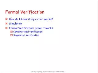
Detecting Design Faults • To check the new implementation for functional correctness, we need: • a reference description: • either a specification • or a previous “golden” implementation. • a new implementation, resulting from • a refinement (synthesis) of the specification • or an optimization of the reference implementation. • a correctness relation which has to be established between the two specifications • (e.g. behavioral correctness).
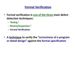
Hardware Verification • Definition: Hardware verification • is the proof that a circuit or a system (the implementation) behaves according to a given set of requirements (the specification). • Formal verification • uses mathematical reasoning to prove that an implementation satisfies a specification • Consideration of all cases is implicit in formal verification.
Funct. Spec RTL Logic Synth. Gate-level Net. Floorplanning …. Formal Verification
Simulation vs. FV • FV uses extensive memory and long run time • Applicable to moderate-size circuits (e.g. blocks or modules)
Formal Verification Methods • Equivalence Checking • Compares optimized/synthesized model against original model • Model Checking • Checks if a model satisfies a given property • Theorem Proving • Proves implementation is equivalent to specification in some formalism
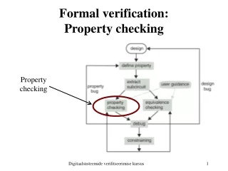
What is Model Checking? • Model Checking (Property Checking): • An automatic technique for verifying finite-state reactive systems, (such as sequential digital circuits or communication protocols). • A reactive FSM is an FSM whose inputs come from the environment. • For checking that a desired property holds in a finite state model of a system • Was pioneered by Edmund Clarke, professor in the CS Dept of CMU, in 1981 • (E.M. Clarke and E.A. Emerson. "Synthesis of Synchronization Skeletons for Branching Time Temporal Logic", in Logic of Programs workshop, Yorktown Heights, NY, May 1981.). reference: Lectures by Karsten Schmidt, Dong Wang Sergey Berezin, Carnegie Mellon University, Jeannette M. Wing
What is Model Checking? (cont.) • Relies on exhaustive state space search. • exhaustive state space search is guaranteed to terminate, as the model is finite. • Major challenge: • To fight state-explosion problem • Can uncover subtle design errors • Can handle large state spaces (10^120) • Quicker to start testing • as it does not require vectors or a testbench. • Successfully used to find bugs in published standards
What is Model Checking? (cont.) • Typically used during RTL code development to debug the RTL model prior to synthesis. • Used concurrently with and/or prior to simulation. • FormalCheck is the name of Cadence’s Model Checking tool. • Currently the dominant formal verification tool.
How does Model Checking work? Finite State Model Model Checker System meets or not Properties
Model Checking Output Space Model-based verification P1 Simulation-based verification P2 P3 : Design Points verified : Properties verified • Sim-based:checks one output point at a time, • FV:checks a group of output points at time. • Idea:Search the entire state space for important points: (i.e. points that fail the property)
Process of Model Checking • Modeling: • convert a design (hardware or software) into a formalism accepted by a model checker • Specification: • to state the properties as golden behavior • use temporal logic to assert how the behavior of the system evolves over time • Verification: • automatic process Reference: J. R. Burch, E. M. Clarke, K. L. McMillan, D. L. Dill, “Sequential circuit verification using symbolic model checking”, Proc. 27th ACM/IEEE Design Automation Conf., June 1990.
Classification of property specification • Functional correctness: • Does the encoder correctly encode? • Does the multiplier multiply? • Temporal behavior: • Does the bus master start the bus access in 6 clocks after it is granted? • Safety properties: • At a traffic intersection, are the traffic lights for both paths green? • Does the elevator door only open after the elevator has come to a complete standstill at some floor? • Liveness properties: • Does the traffic light become green eventually? • Fairness properties : • Is every requesting master eventually granted by the bus arbiter
Model Checking • Property is a partial specification of the design, • essentially a duplicate description of the design (redundancy in specification). • As equally prone to errors as the design. • Practical Issues: • ~70% of verification time is spent on getting correct constraints! • Debugging is difficult when the property is written in a language other than that of the design. • e.g. property in SystemVerilog, design in Verilog. • Debugging failures in a property specification has the same difficulty as any other debugging activities.
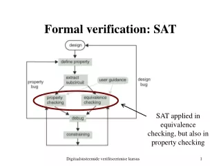
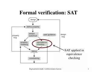
Equivalence Checking • Two Methods: • Combinational Equivalence Checking • Sequential Equivalence Checking
Equivalence Checking • Combinational Equivalence Checking: • The functions of the two circuits to be compared are converted into canonical representations of Boolean functions, typically Binary Decision Diagrams (BDDs). • The BDDs are then structurally compared. • Unable to compare the RTL model with a behavioral model.
1 outputs inputs 2 1’ inputs outputs 2’ Logic Equivalence Checking • Task : Check functional equivalence of two designs • Inputs • Reference (golden) design • Optimized (synthesized) design • Logic segments between registers, ports or black boxes • Output • Matched logic segment equivalent/not equivalent • This is achieved by dividing the model into logic cones between registers, latches or black-boxes. • The corresponding logic cones are then compared between original and optimized models. 1 = 1’ ? 2= 2’ ? Equivalence result Reference design Optimized design
F F T T Combinational Equivalence Checking BDD (Binary Decision Diagram) Circuit/Implementation (comb. ckt) Circuit/Implementation A isomorphic ? Circuit/Implementation B
Sequential Equivalence Checking • Sequential Equivalence checking: • verifies the equivalence between two sequential designs at each valid state. • This is achieved by creating a finite state machine representation of the two systems and checking whether a state can be reached from initial states where two corresponding outputs of the models differ. • Can verify the equivalence between RTL and the behavioral model. • Suffers from the state space explosion problem due to creating a full finite state representation of two systems.
Sequential Equivalence Checking • Common input A drives the two Models • State Vectors are held in S1 and S2 and initialised to a common value – all zeroes for instance. • The outputs Z1 and Z2 are compared by XORing them • If E remains zero then the two models are equivalent • The state space explosion rules out this approach
Boolean Equivalence Checking(BEC) • Assuming that the two FSMs are the same with same encoding of states it is enough to prove that the two combinational logics are equivalent • Equivalence is established without having to do statespace exploration • Next state logic and output logic are checked for equivalence. E1 and E2 should remain zero. • Simulation based method won’t be able to exhaustively check even this restricted problem
xy x r xx xy pr ps pt x p a = × a y s aa y b b b bb q yy yx qt qr qs y t yy bb FSM Equivalence Checking • Task : Check if implementation is equivalent to spec • Inputs • FSM for specification (Ms) • FSM for implementation (Mi) • Output • Do Mi and Ms give same outputs for same inputs ? • Idea (Devadas, Ma, Newton ’87) • Compute Mi×Ms • Qf(Mi×Ms) = States which have different outputs for Mi and Ms • Check if any state in Mi×Ms is reachable.
Applications of EC • Applications: • Before and after scan insertion: • to make sure that adding scan chain does not alter functionality. • Ensure integrity of a layout vs. RTL version • First circuit extraction to transistor netlist. • Prove that ECO changes are restricted to the scope intended.
Assumptions / Background theories / Inference rules Theorem Prover Proof Goal decomposition | proof Theorem Proving • Task : • Prove implementation is equivalent to spec in given logic • Inputs • Formula for specification in given logic (spec) • Formula for implementation in given logic (impl) • Assumptions about the problem domain • Example : Vdd is logic value 1, Gnd is logic value 0 • Background theory • Axioms, inference rules, already proven theorems • Output • Proof for spec = impl Manual Automated
Theorem Proving • Example • CMOS inverter (Gordon’92) • Using higher order logic • Assumptions • Vdd(y) := (y=T) • Gnd(y) := (y=F) • Ntran(x,y1,y2) := (x->(y1=y2)) • Ptran(x,y1,y2) := (┐x->(y1=y2)) • Impl(x,y) := ∃ w1, w2. Vdd(w1) Λ Ptran(x,w1,y) Λ Ntran(x,y,w2) Λ Gnd(w2) • Spec(x,y) := (y=┐x) • Proof • Impl(x,y) = ….. (assumption / thm / axiom) = ….. (assumption / thm / axiom) = ….. (assumption / thm / axiom) = Spec(x,y) Vdd w1 x y w2 Gnd CMOS inverter
Theorem Proving • Example • AND Logic • 4 steps: • Specify the implementation of the AND gate, • Specify the behavioral models for the NAND and NOT gates, • Specify the intended behavior of the AND gate, • Prove that the implementation satisfies its intended behavior. Implementation of AND
Drawbacks of Theorem Proving • Not easy to deploy in industry • Most designers don’t have background in math logic • Models must be expressed as logic formulas • Limited automation • Extensive manual guidance to derive proof sub-goals
Theorem Proving • Theorem prover is less automatic than a model checker (more of an assistance to the user): • User: • assembles relevant info for the tool, • sets up intermediate goals (i.e. lemmas) • Tool: • Attempts to achieve the intermediate goals based on input data. • Effective use of it requires • a solid understanding of the internal operations of the tool and • familiarity with the mathematical proof process.
Assertion-Based Verification • An assertion is a statement that a specific condition, or sequence of conditions, in a design must be true. • Describe expected or unexpected conditions (assertions) in device under test (DUT) • Specialized languages (e.g. e, Sugar/PSL) • Language extensions or features (Open Verification Library (OVL), SystemVerilog) • Check to make sure that conditions are satisfied • Dynamically during simulation • Statically using formal • Hybrid • Assertions could be independent & separated from design description
Assertion-based Verification- Usage modes • Static formal • no pattern required spec. describe the behavior (assertions) describe the design assertions DUT check engine exhaustively proven (no violation) N violate ? Y an example of an errant behavior (counterexample)
Assertion-based Verification- Usage modes • Dynamic check • similar as simulation, but check the properties from assertions • input pattern required • the proof depends on the coverage of input pattern spec. describe the behavior (assertions) describe the design assertions DUT test pattern 0100111x0 11111000 01010101 100101 simulation violation alert
Applicability • Well accepted techniques in industry • Simulation with assertions • Static assertions • Equivalence checking
Applicability • Wrong assumptions: • A puristic claim: • A verification run was considered to be successful only if the complete system had been verified. • Facts: • The systems are too large • If it can be shown that verification is able to find more faults than simulation in the same time, then it is cost-effective and should be used. • Methodology: only the critical parts of the system are verified. • A complete system verification is even unnecessary in many cases. (the verification of well-structured and simple parts is not necessary). • A complete formalization of the implementation is intractable. • Verification tools have to be used together with simulation
Applicability • Wrong assumptions: • Formal methods can guarantee the perfectness of systems • Facts: • can significantly enhance the trust, but not able to guarantee flawlessness. • Reasons: • Only makes correctness statements with regard to a formal specification which can be faulty itself. • Faults in verification program. • Only design faults but not fabrication faults or faults during system usage.
Tools • Verification Languages: • "e". • Synopsys Vera : • SystemC SCV • Equivalence Checkers: • Cadence Verplex : • Synopsys Formality : • Mentor FormalPro : • Prover eCheck : • homebrew EC • Assertion Languages: • IBM Sugar/PSL • 0-in Checkerware • Verplex OVL • System Verilog SVA • Synopsys Vera OVA
References • W. Lam, Hardware Design Verification, Simulation and Formal Method-Based Approaches, Prentice-Hall, 2005. • Kropf, T., Introduction to Formal Hardware Verification, Springer, 1999. • D. Gajski and S. Abdi, "System Debugging and Verification: A New Challenge," Verify 2003, Tokyo, Japan, November 20, 2003.