S2 Hardware Pulsar Injections
230 likes | 370 Views
S2 Hardware Pulsar Injections. LSC Pulsar Group and P Shawhan, S Marka, and S Koranda presented by B Allen, R Dupuis, N Christensen, and X Siemens. Provides end-to-end validation of search code: Gain confidence about tricky things like floating point dynamic range in filtering process

S2 Hardware Pulsar Injections
E N D
Presentation Transcript
S2 Hardware Pulsar Injections LSC Pulsar Group and P Shawhan, S Marka, and S Koranda presented by B Allen, R Dupuis, N Christensen, and X Siemens LSC WIDE COLLOQUIUM
Provides end-to-end validation of search code: Gain confidence about tricky things like floating point dynamic range in filtering process Helps algorithm/code developers in testing Provide a fixed point of reference to return to Challenges in the pulsar case: Realistic signals must last for hours (~107 cycles). This is unlike the burst (seconds) and inspiral (tens of seconds) case. Would like to avoid the “SB” scenario where the simulated signal dominates the data Getting the correct initial phase relationship at the different detector sites can be tricky (specifics later) Simpler in pulsar case: Calibration: signal is at a “single” frequency Why Do Hardware Injections? LSC WIDE COLLOQUIUM
Signal is sum of two different pulsars, P1 and P2 S2 Pulsar Injection Parameters P1: Constant Intrinsic Frequency Sky position: 0.3766960246 latitude (radians) 5.1471621319 longitude (radians) Signal parameters are defined at SSB GPS time 733967667.026112310 which corresponds to a wavefront passing: LHO at GPS time 733967713.000000000 LLO at GPS time 733967713.007730720 In the SSB the signal is defined by f = 1279.123456789012 Hz fdot = 0 phi = 0 A+ = 1.0 x 10⁻²¹ Ax = 0 [equivalent to iota=pi/2] P2: Spinning Down Sky position: 1.23456789012345 latitude (radians) 2.345678901234567890 longitude (radians) Signal parameters are defined at SSB GPS time: SSB 733967751.522490380, which corresponds to a wavefront passing: LHO at GPS time 733967713.000000000 LLO at GPS time 733967713.001640320 In the SSB at that moment the signal is defined by f=1288.901234567890123 fdot = -10-8 [phase=2 pi (f dt+1/2 fdot dt^2+...)] phi = 0 A+ = 1.0 x 10⁻²¹ Ax = 0 [equivalent to iota=pi/2] LSC WIDE COLLOQUIUM
12 hours of strain data was produced (with overall 1021 normalization factor) using LAL routines: 144 files (5 minutes each) were produced. Each file contains 16384*300+1 4-byte IEEE 754 floats: Key 1234.5 (4 bytes) Sample 0 xxxxxx (4 bytes) Sample 1 yyyyyy (4 bytes) … Time range was 00:00 –12:00 UTC April 10th The 2.8 GB of injection data was shipped to each site More details of signals in LIGO DCC: LIGO-G030479-00-Z How was simulated signal made? S2_pulsar_LHO_733968013.dat S2_pulsar_LHO_733968313.dat S2_pulsar_LHO_733968613.dat … and so on. LSC WIDE COLLOQUIUM
Simulated strain: Detector Response Function April 10th 10:00 UTC is: LHO: 2 am April 10th LLO: 4 am April 10th simulated source is passing near a zero of the antenna pattern. April 10th 04:00 UTC is: LHO: 8 pm April 9th LLO: 10 pm April 9th LSC WIDE COLLOQUIUM
More than 9 hours of pulsar injections into L1, H1 and H2 Start 18:19 PDT on April 9 Stop 04:03 PDT on April 10 Instruments were in lock for almost the entire time Pulsar plus calibration line summed into DARM_CTRL ETM_X and ETM_Y used for other injections Strain/DARM_CTRL calibrations worked out at 1284 Hz, halfway between two signals.NOTE: THESE WERE SUBSEQUENTLY REVISED FOR H1 AND H2 – SO AT THOSE DETECTORS THE OVERALL STRAIN FACTOR WAS NOT 1.e-21! Injections started at 733974613 (01:50:00 UTC April 10) and continued until 734007889 (11:04:36 UTC April 10) with some minor interruptions (loss of lock, realignment, computer restarted because of lack of memory). How and When? LSC WIDE COLLOQUIUM
For each signal all parameters were successfully inferred (except a constant 90 degrees phase shift) Four plots were produced for each signal: posterior probability density function of h0 given the data (marginalized over the other parameters) confidence contour plot of \cos\iota vs h0 with levels at 67%, 95%, 99%, and 99.9% confidence contour plot of polarisation angle \psi vs h0 with levels at 67%, 95%, 99%, and 99.9% confidence contour plot of phase \phi_0 vs h0 with levels at 67%, 95%, 99%, and 99.9% Coherent analysis using data from all sites showed that phase was conserved between sites Full results (with larger images) are posted at http://www.astro.gla.ac.uk/users/rejean/lsc/S2injections (lsc/lsconly) Time Domain Bayesian Analysis LSC WIDE COLLOQUIUM
L1: Results for signal P1 p(h0, | Bk) p(h0,cos | Bk) p(h0,0| Bk) p(h0| Bk) H1: H2: LSC WIDE COLLOQUIUM
Results for signal P2 p(h0, | Bk) p(h0,cos | Bk) p(h0,0| Bk) p(h0| Bk) L1: H1: H2: LSC WIDE COLLOQUIUM
p(a|all data) = p(a|H1) p(a|H2) p(a|L1) Joint Coherent Analysis Signal P1 Signal P2 all IFOs individual IFOs LSC WIDE COLLOQUIUM
Parameters : f0, cos(i), y, h0, and then df Tested on synthesized data (4 and 5 parameters) Tested on the S2 Injected Signals (4 parameters) Use likelihood and priors of the time-domain search as MCMC starting point. df uncertain to 1/60 Hz. For a 5 Hz search, run on 300 nodes 10 hours cpu for 10 days of data Markov Chain Monte Carlo Results 4 and 5 Parameter Search Works WellAnd Has Been Tested LSC WIDE COLLOQUIUM
4 Parameters: S2 Injection: It Works! Signal 1 as seen in H1 above. Exact match with time domain search. Full results posted at http://physics.carleton.edu/Research/ligo/S2injectCW.html Found h0, y, and cos(i), but f0 off due presumably to a time definition LSC WIDE COLLOQUIUM
Signal 1 at H1 Signal 1: Parameters of injected signal: RA = 5.1471621319 rad DEC = 0.3766960246 rad f0 = 1279.123456789012 Hz fdot = 0.0 psi = 0.0 phi=0.0 cos(iota)=0.0 h0 = 2.0e-21 (± calibration errors) MCMC Result (h0 scaled by 10-22) The Statistics Are: Mean Standard Deviation h0 20.97711 1.44419 psi -0.02704 0.02424 phi -0.66802 0.03438 cosiota -0.04865 0.02474 Quantiles for each variable: 2.5% 97.5% h0 18.17624 23.817896 psi -0.07318 0.019197 phi -0.73427 -0.601182 cosiota -0.09867 -0.001396 LSC WIDE COLLOQUIUM
Signal 2 at L1 Signal 1 as seen in L1 above. Exact match with time domain search. LSC WIDE COLLOQUIUM
Signal 1 at L1 Signal 1: Parameters of injected signal: RA = 5.1471621319 rad DEC = 0.3766960246 rad f0 = 1279.123456789012 Hz fdot = 0.0 psi = 0.0 phi=0.0 cos(iota)=0.0 h0 = 2.0e-21 (± calibration errors) MCMC Results (h0 scaled by 10-22) The statistics are: Mean Standard Deviation h0 19.00456 1.44050 psi -0.08483 0.03439 phi -0.82187 0.04071 cosiota -0.07484 0.03583 Quantiles for each variable: 2.5% 97.5% h0 16.2522 21.889774 psi -0.1460 -0.011781 phi -0.9026 -0.743842 cosiota -0.1473 -0.005469 LSC WIDE COLLOQUIUM
Signal 2 at H2 Signal 2 as seen in H2 above. Exact match with time domain search. LSC WIDE COLLOQUIUM
Signal 2 at H2 MCMC Results (h0 scaled by 10-22) The statistics are: Mean SD h0 19.132891 0.91848 psi -0.008155 0.02172 phi -0.753110 0.02425 cosiota 0.061423 0.02135 Signal 2: Parameters of injected signal: RA = 2.345678901234567890 DEC = 1.23456789012345 f0 = 1288.901234567890123 Hz fdot = -1.0e-8 Hz/s psi = 0.0 h0 = 2.0e-21 (± calibration errors) phase = 0.0 cos(iota)=0.0 Quantiles for each variable: 2.5% 97.5% h0 17.24495 21.02338 psi -0.05211 0.03266 phi -0.80178 -0.70678 cosiota 0.02091 0.10527 LSC WIDE COLLOQUIUM
Parameters : df, dfdot, f0, cos(i), psi, and h0 Test on synthesized data has commenced Different Technique - “Delayed Rejection in Reversible Jump Metropolis-Hastings”, plus other tricks. Will soon test on S2 injected signal 2 where dfdot is non-zero New manpower - John Veitch @ Glasgow 6 Parameter Search: Road to a SN1987A Search LSC WIDE COLLOQUIUM
6 Parameter Search Generated PDFs from the parameters h0, df, and dfdot. In this example from the 6 parameter problem the true values for the critical parameters were h0=10.0, df = 0.0078125, and dfdot = 2x10⁻¹⁰. The priors we uniform -10-9Hz/s<dfdot<10-9 Hz/s and -1/60 Hz < df < 1/60 Hz LSC WIDE COLLOQUIUM
S2 Frequency DomainInjection Results The signal in the data (green 60s SFTs, red 1800s SFTs) Signal I Signal I Hz Hz Signal II Signal II Hz Hz LSC WIDE COLLOQUIUM
Results LSC WIDE COLLOQUIUM
FD Conclusions • Still have problems with phase of the signal … • 1800s SFTs (which I did not show results for) have equally good results (they are calibrated with calibration factors averaged every 30 mins) • Overall results are very encouraging LSC WIDE COLLOQUIUM
The Pulsar Group will to provide a fast real-time function that can be called, which will return h(t). Will be used to do pulsar injections during entire S3 run (~5 pulsars, parameters TBD). Uta Weiland (GEO Hannover) is writing a routine for this purpose for GEO pulsar injections. Can only inject 1 pulsar. What about S3? LSC WIDE COLLOQUIUM