Regression Analyses
This comprehensive overview of multiple regression covers its framework, assumptions, and practical applications. Multiple regression is a powerful statistical method used to predict a dependent variable (DV) from multiple independent variables (IVs). We explore the general regression equation, the significance of beta weights, and the challenges like multicollinearity. Additionally, we discuss the importance of correctly specifying models, ensuring the independence of errors, and how to maximize the explained variance. Ideal for researchers and students seeking deeper insights into regression analysis.

Regression Analyses
E N D
Presentation Transcript
Multiple Regression • Multiple IVs • Single DV (continuous) • Generalization of simple linear regression • Y’ = b0 + b1X1 + b2X2 + b3X3...bkXk • Where k is the number of predictors • Find solution where Sum(Y-Y’)2 minimized • Do not confuse size of bs with importance for prediction • Can standardize to get betas, which can help determine relative importance
Why use Multiple Regression? • Prediction – allows prediction of change in the D.V. resulting from changes in the multiple I.V.s • Explanation – enables explanation of the variate by assessing the relative contribution of each I.V. to the regression equation • More efficient than multiple simple regression equations • Allows consideration of overlapping variance in the IVs
When do you use Multiple Regression? • When theoretical or conceptual justification exists for predicting or explaining the D.V. with the set of I.V.s • D.V. is metric/continuous • If not, logistic regression or discriminant analysis
Variance in Y Y e a residual variance X1 c b Variance in X1 X2 Variance in X2 Multiple Regression
Assumptions • DV is continuous and interval or ratio in scale • Assumes multivariate normality for random IVs • Assumes normal distributions and homogeneity of variance for each level of X for fixed IVs • No error of measurement • Correctly specified model • Errors not correlated • Expected mean of residuals is 0 • Homoscedasticity (error variance equal at all levels of X) • Errors are independent/no autocorrelation (error for one score not correlated with error for another score) • Residuals normally distributed
Multiple regression represents the construction of a weighted linear combination of variables: • The weights are derived to: • Minimize the sum of the squared errors of prediction: • (b) Maximize the squared correlation (R2) between the original outcome variables and the predicted outcome variables based on the linear combination.
Y y-y` X
Multiple R • R is like r except it involves multiple predictors and R cannot be negative • R is the correlation between Y and Y’ where • Y’ = b0+b1X1 + b2X2 + b3X3...bkXk • R2 tells us the proportion of variance accounted for (coefficient of determination)
An example . . . Y = Number of job interviews X1 = GRE score X2 = Years to complete Ph.D. X3 = Number of publications N = 500
Predicting Interviews Variance in Interviews Variance in Time to Graduate e f c residual variance d a b Variance in GRE Variance in Pubs
Regression with SPSS • From Analyze Menu • Choose Regression • Choose Linear REGRESSION /MISSING LISTWISE /STATISTICS COEFF OUTS R ANOVA /CRITERIA=PIN(.05) POUT(.10) /NOORIGIN /DEPENDENT interviews /METHOD=ENTER years to complete gre pubs /SCATTERPLOT=(*ZPRED ,*ZRESID) .
The variance that is maximized in the derivation of the regression weights. The error that is minimized in the derivation of the regression weights: the standard deviation of errors of prediction.
The error that is minimized in the derivation of the regression weights: the variance of errors of prediction.
The weight, b The weight, b, if variables are standardized.
Output from SPSS Significance of Beta weights.
Multicollinearity • Addition of many predictors increases likelihood of multicollinearity problems • Using multiple indicators of the same construct without combining them in some fashion will definitely create multicollinearity problems • Wreaks havoc with analysis • e.g., significant overall R2, but no variables in the equation significant • Can mask or hide variables that have large and meaningful impacts on the DV
Multicollinearity Multicollinearity reflects redundancy in the predictor variables. When severe, the standard errors for the regression coefficients are inflated and the individual influence of predictors is harder to detect with confidence. When severe, the regression coefficients are highly related. var(b)
The tolerance for a predictor is the proportion of variance that it does not share with the other predictors. The variance inflation factor (VIF) is the inverse of the tolerance.
Multicollinearity Remedies: (1) Combine variables using factor analysis (2) Use block entry (3) Model specification (omit variables) (4) Don’t worry about it as long as the program will allow it to run (you don’t have singularity, or perfect correlation)
Incremental R2 • Changes in R2 that occur when adding IVs • Indicates the proportion of variance in prediction that is provided by adding Z to the equation • It is what Z adds in prediction after controlling for X in Z • Total variance in Y can be broken up in different ways, depending on order of entry (which IVs controlled first) • If you have multiple IVs, change in R2 strongly determined by intercorrelations and order of entry into the equation • Later point of entry, less R2 available to predict
Other Issues in Regression • Suppressors (one IV correlated with the other IV but not with the DV; switches in sign) • Empirical cross-validation • Estimated cross-validation • Dichotomization, Trichotomization, Median splits • Dichotomize one variable reduces max r to .798 • Cost of dichot is loss of 1/5 to 2/3 of real variance • Dichot on more than one variable can increase Type I error and yet can reduce power as well!
Tests: a + b + c + d + e + f against area g (error) Get this from a simultaneous regression or from last step of block or hierarchical entry. Other approaches may or may not give you an appropriate test of overall R2, depending upon whether all variables are kept or some omitted. Significance of Overall R2 X Y a g b e c d W f Z
Significance of Incremental R2 Step 1: Enter X Change in R2 tests: a + b + c against area d + e + f + g At this step, the t test for the b weight of X is the same as the square root of the F test if you only enter one variable. It is a test of whether or not the area of a + b + c is significant as compared to area d + e + f + g. X Y a g b e c d f
Significance of Incremental R2 Step 2: Enter W X Y Change in R2 tests: d + e against area f + g At this step, the t test for the b weight of X is a test of area a against area f + g and the t test for the b weight of W is a test of area d + e against area f + g. a g b e c d f W
Significance of Incremental R2 Step 3: Enter Z Change in R2 tests: f against g X Y a At this step, the t test for b weight of X is a test of area a against area g, the t test for the b weight of W is a test of area e against area g, and the t test for the b weight of Z is a test of area f against area g. These are the significance tests for the IV effects from a simultaneous regression analysis. No IV gets “credit” for areas b, c, d in a simultaneous analysis. g b e c d f W Z
Hierarchical RegressionSignificance of Incremental R2 Enter variables in hierarchical fashion to determine R2 for each effect. Test each effect against error variance after all variables have been entered. X Y a g b e Assume we entered X then W then Z in a hierarchical fashion. c d f W Tests for X: areas a + b + c against g Tests for W: areas d + e against g Tests for Z: area f against g Z
Significance test for b or Beta In final equation, when we look at the t tests for our b weights we are looking at the following tests: X Y a Tests for X: Only area a against g Tests for W: Only area e against g Tests for Z: Only area f against g That’s why incremental or effect R2 tests are more powerful. g b e c d f W Z
Methods of building regression equations • Simultaneous: All variables entered at once • Backward elimination (stepwise): Starts with full equation and eliminates IVs on the basis of significance tests • Forward selection (stepwise): Starts with no variables and adds on the basis of increment in R2 • Hierarchical: Researcher determines order and enters each IV • Block entry: Researcher determines order and enters multiple IVs in single blocks
Simultaneous Y a g • Variable X & Z together • predict more than W • Variable W might be • significant, X & Z are not • Betas are partialled, so • beta for W larger than X • or Z X i f d b e h W c Z • Simultaneous: All variables entered at once • Significance tests and R2 based on unique variance • No variable “gets credit” for area g • Variables with intercorrelations have less unique variance
Backward Elimination Y a g X i d f e b h W c Z • Starts with full equation and eliminates IVs • Gets rid of least significant variable (probably X), then tests remaining vars to see if they are signif • Keeps all remaining significant vars • Capitalizes on chance • Low cross-validation
Forward Selection Y a g X i f d b e h W c Z • Starts with no variables and adds IVs • Adds most unique R2 or next most significant variable (probably W because gets credit for area i) • Quits when more vars are not significant • Capitalizes on chance • Low cross-validation
Hierarchical (Forced Entry) Y a g X f d i b e h W c Z • Researcher determines order of entry for IVs • Order based on theory, timing, or need for stat control • Less capitalization on chance • Generally higher cross-validation • Final model based on IVs of theoretical importance • Order of entry determines which IV gets credit for area g
Order of Entry • Determining order of entry is crucial • Stepwise capitalizes on chance and reduces cross-validation and stability of your prediction equation • Only useful to maximize prediction in a given sample • Can lose important variables • Use the following: • Logic • Theory • Order of manipulations/treatments • Timing of measures • Usefulness of the regression model is reduced as the k (number of IVs) approaches N (sample size) • Best to have at least 15 to 1 ratio or more
Interpreting b orb • B or b is raw regression weight b is standardized (Scale invariant) • At a given step, size of b or b influenced by order of entry in a regression equation • Should be interpreted at entry step • Once all variables are in the equation, bs and bs will always be the same regardless of the order of entry • Difficult to interpret b or b for main effects when interaction in equation
Regression: Categorical IVs • We can code groups and use to analyze data (e.g., 1 and 2 to represent females and males) • Overall R2 and significance tests for full equation will not change regardless of how we code (as long as orthogonal) • Interpretation of intercept (a) and slope (b or beta weights) WILL change depending on coding • We can use coding to capture effects of categorical variables
Regression: Categorical IVs • Total # codes needed is always # groups -1 • Dummy coding • One group assigned 0s. b wts indicate mean difference of groups coded 1 compared to the group coded 0 • Effect coding • One group assigned -1s. b wts indicate mean difference of groups coded 1 to the grand mean • All forms of coding give you the same overall R2 and significance tests for total R2 • Difference is in interpretation of b wts
Dummy Coding • # dummy codes = # groups – 1 • Group that receives all zeros is the reference group • Beta = comparison of reference group to group • represented by 1 • Intercept in the regression equation is mean of the • reference group
Effect Coding • # contrast codes = # groups – 1 • Group that receives all zeros in dummy coding now gets all -1s • Beta = comparison of the group represented by 1 to the grand mean • Intercept in the regression equation is the grand mean
Regression with Categorical IVs vs. ANOVA • Provides the same results as t tests or ANOVA • Provides additional information • Regression equation (line of best fit) • Useful for future prediction • Effect size (R2) • Adjusted R2
Regression with Categorical Variables - Syntax Step 1. Create k -1 dummy variables Step 2. Run regression analysis with dummy variables as predictors REGRESSION /MISSING LISTWISE /STATISTICS COEFF OUTS R ANOVA /CRITERIA=PIN(.05) POUT(.10) /NOORIGIN /DEPENDENT fiw /METHOD=ENTER msdum1 msdum2 msdum3 msdum4 msdum5 .
Adjusted R2 • There may be “overfitting” of the model and R2 may be inflated • Model may not cross-validate shrinkage • More shrinkage with small samples (< 10-15 observations per IV)
Example: Hierarchical Regression Example. Number of children, hours in family work and sex as predictors of family interfering with work REGRESSION /MISSING LISTWISE /STATISTICS COEFF OUTS R ANOVA CHA /CRITERIA=PIN(.05) POUT(.10) /NOORIGIN /DEPENDENT fiw /METHOD=ENTER numkids /METHOD=ENTER hrsfamil /METHOD=ENTER sex .