The Static and Dynamic Properties of Liquids and Disordered Systems

1. The Static and Dynamic Properties of Liquids and Disordered Systems Walter Kob University of Montpellier France 2018 Summer School on Soft Matter and Biophysics INS, Shanghai, China July 1 - 5, 2018

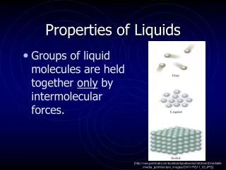
2. Motivation • Phase diagram of a simple system • Gas phase: - Particles are far apart and thus do not interact with each other - disorder and no correlation  universal gas laws • High school physics • Crystalline phase • Particles are close to each other • strong interactions • particles are on a regular lattice • particles are close to minimum of potential energy one can make a harmonic approximation phonons • undergraduate physics • Liquids: Particles interact strongly with each other; correlation on small length scales but disorder on large length scales; no small parameter  Very difficult

3. Motivation: Typical structures • Structure of most disordered systems is very complex

4. Outline of the Lectures • Literature • Characterizing the structure • Calculating the structure: Models; theoretical calculations • Characterizing the dynamics • Calculating the dynamics: Models; theoretical calculations

5. Literature • N. H. March and M. P. Tosi, Atomic Dynamics in Liquids (Dover, New York, 1976). • J. P. Boon and S. Yip, Molecular Hydrodynamics (Dover, New York, 1980). • U. Balucani and M. Zoppi, Dynamics of the Liquid State (Clarendon, Oxford, 1994). • J.-P. Hansen and I. R. McDonald, Theory of Simple Liquids (Academic, London, 2013). • P.A. Egelstaff, An Introduction to the Liquid State (Clarendon, Oxford, 1992). • M. Rubinstein and R. H. Colby, Polymer Physics (Oxford University Press, 2003). • J.L. Barrat and J.-P. Hansen, Basic Concepts for Simple and Complex Liquids (Cambridge, 2003). • K. Binder and W. Kob, Glassy Materials and Disordered Solids (World Scientifc, 2011)

6. Characterizing the structure • Radial distribution function • Static structure factor • Energy and pressure equation

7. Radial distribution function: 1 • N classical particles with coordinates ri, i = 1, 2, …, N Potential energy: • Hamiltonian H: • Canonical average of an arbitrary phase space variable A • Z is the partition function: :=kBT(kB=Boltzmann constant=1.38 x 1023m2 kg s-2 K-1).

8. Radial distribution function: 2 • Define local density (r) • define the density-density correlation function G(r) •  = N/V is the particle density ; function g(r) is defined by the last equation  if there is a particle at the origin one finds on average n(r) = 4r2g(r) other particles at a distance r. • g(r) converges to 1-1/N for r large

9. Radial distribution function: 3 • Example: Lennard-Jones fluid • g(r) is zero at small r because of repulsion between particles  correlation hole • g(r) allows to understand the shell structure of liquids with decreasing correlation at large distances • NB: For soft particles the correlation hole can be weak

10. Radial distribution function: 4 • Usually one has multicomponent systems  need to generalize definitions;  species • local density of species  • Partial pair distribution functions g(r): NB: Symmetry

11. Static Structure factor S(k) • Consider the spatial Fourier transform of (r): k: wave-vector • define the static structure factor • For a homogeneous system one has • inverse Fourier transform • Experiments: neutron or X-ray scattering

12. Static Structure factor S(k): 2 • For isotropic systems S(k) depends only on the module k=|k|  integration over sphere • Note that for k0, S(q) does not go to zero; one has T: Compressibility

13. Multicomponent systems • So far: One component system; real systems have often many components (type of atoms)  need to generalize formalism Partial structure factors NB: Symmetry S(k) = S(k) • Usually experiments cannot access S(k) but only the weighted sum over the partial structure factors Example neutron scattering b : neutron scattering length • X-ray scattering: replace b by a function b(k) (see www) • To access S(k) one must make isotope substitution

14. Multicomponent systems: 2 • Neutron scattering and X-ray scattering can give quite different Example: Glass Na2O-SiO2-B2O3 NB: Symmetry S(k) = S(k) Peaks are at different positions; meaning is sometimes not clear; position of peak does not mean that there is a relevant distance in real space

15. Compare g(r) and S(q) • From a mathematical point of view g(r) and S(k) contain the same information. BUT Information that is clearly visible in real space might be obscured in reciprocal space

16. Energy Equation • g(r ) is not only useful for characterizing the structure but allows to express the energy • We assume that the interactions between the particles are given by a pair potential v(r) The average potential energy of the system is then ZN(V,T): configurational part of the partition function

17. Energy Equation: 2 • Make integral over angular part gives the “energy equation” Similar reasoning for pressure; statistical mechanics gives On obtains: Pressure equation For hard spheres:

18. Calculating the structure: Models; theoretical calculations • Polymers and random walks • Direct correlation function • Closer relations: From the interaction to the structure

19. Polymers and Random Walks • Polymers: Long chain of identical units; “units” can be complex • Simplest model for a polymer: n + 1 monomers that are bonded with n bonds with bond length l • End-to-end distance • Mean squared end-to-end distance: since Thus Real polymers: Monomers have excluded volume interactions  polymer swells Equivalently Polymer is a fractal with dimension 1/ NB: Compact polymers

20. Polymers: Structure factor • Static structure factor of a single polymer is given by Use and convert sum into integral

21. Polymers: Structure factor: 2 • Integral gives Mean squared radius of gyration For Gaussian chain one has Limits: Thus with

22. Polymers: Structure factor: 3 Isolated polymer chain in vacuum Isolated polymer chain in polymer melt

23. Direct Correlation Function • g(r) shows various peaks that are due to the interactions between the particles. • These interactions can be decomposed into a direct correlation and an indirect correlation. So we define the total correlation function  h(r) goes to zero if r is large • We write which is an implicit definition of the direct correlation function c(r) Ornstein-Zernike equation

24. Direct Correlation Function: 2 Fourier transformation Connection with S(k):  If we know S(k) we can obtain C(k)

25. Closure relation • To get h(r) (and thus g(r)) we need an additional equation that connects h(r) or c(r) to the pair potential v(r). This additional equation is called “closure relation“ • g(r) is not negative  we can write it as w(r) is the “potential of mean force". We write w(r) as The “bridge function” b(r) is unknown! with • In the following we will set b(r)=0

26. Percus-Yevick approximation Make Taylor expansion of exp((r)) and keep first 2 terms: and thus This equation and the Ornstein-Zernike equation can be solved (numerically) For hard sphere system the PY can be solved analytically (see later)

27. Hypernetted chain approximation One only sets b(r )=0 and not further approximations and thus This equation and the Ornstein-Zernike equation can be solved (numerically) Usually the HNC is more accurate than the PY equation since one makes one approximation less

28. PY equation for hard spheres • For the case of hard spheres it is possible to solve the PY equations analytically (Thiele & Wertheim 1963): Define packing fraction Exact analytical solution: with With the OZ equation this gives the H(k) and thus g(r)

29. Characterizing the Dynamics • General properties of time correlation functions • Velocity auto-correlation function • van Hove correlation function • Intermediate scattering function • Rouse model • Glassy dynamics and mode-coupling theory

30. General properties of time correlation functions • We consider a dynamical variable A(t) which is given by the temporal evolution of the system • Remark 1: The RHS depends on the initial condition, i.e. the state of the system at time t = 0. For ergodic systems this dependence can be neglected; problematic case: glasses • Remark 2: The evolution of the system will depend on the microscopic dynamics (Newtonian dynamics, Brownian dynamics,...) • define a time correlation function between two dynamical variable A(t) and B(t) and denote it by CAB(t’; t’’)

31. Time correlation functions: 2 • If system is ergodic we can replace the thermal average by a time average Stat. mech. vs. Nature • If Hamiltonian H is independent of time CAB(t’; t’’) depends only on t’-t’’ • CAB(t) must be independent of the origin of time • For A=B we have • For t=0 we thus have • Similar calculation gives

32. Time correlation functions: 3 • Bounds on time correlation functions: Recall the Schwarz inequality of mathematics: Assume we have a complex Hilbert space D with an inner product (x, y) for two elements x and y in D. Then one can show that • Apply this to the case Thus we obtain or • For the case B=A we thus have  an autocorrelation function cannot exceed its value at t=0

33. Time correlation functions: 4 • In most case the correlation between two dynamical variables A(t) and B(t) does not go to zero But for mathematical reasons it is useful to have correlation function that go to zero at long times (Fourier-transforms!)  redefine time correlation functions

34. Spectral function • Power spectrum (or spectral function): FT of correlator: • CAB() can be measured directly in experiments (e.g. dielectric constant at frequency ) • One can show that the spectrum of an autocorrelation function is not negative • Proof: Define • The quantity is not negative, i.e.  Limit T  bracket becomes 

35. Spectral function: 2 • The inverse FT gives for the case B = A • differentiate equation 2n times with respect to t gives For t=0 this gives  Moments of the spectral function are directly related to the time derivative of the autocorrelation function at t=0 • If the Hamiltonian is time reversal (e.g. Newtonian dynamics) we can make a Taylor expansion of CAA(t) in term of even power of t: Thus we obtain

36. Velocity auto-correlation function • Example of a time correlation function: The velocity autocorrelation function (VAF) For t = 0 the value of Z(t) follows from the equipartition theorem We can write

37. Velocity auto-correlation function: 2 Square and average

38. Velocity auto-correlation function: 3 • Einstein relation between the diffusion constant and the mean squared displacement • This equality is an example for a Green-Kubo relation, i.e. the connection between a time integral over a correlation function and a transport coefficient. Other examples: stress-stress-correlation  viscosity

39. Van Hove correlation function • Consider the dynamical observable of the local density The van Hove function is now defined as or Split G(r, t) into diagonal and off-diagonal term

40. Van Hove correlation function: 2 “self part of the van Hove function" “distinct part of the van Hove function" One sees that Normalization

41. Van Hove correlation function: 3 • Binary Lennard-Jones mixture “cage effect” • Sodium silicate liquid • Na shows “hopping” motion

42. Van Hove correlation function: 4 • Look at Gs(r,t) instead of 4r2Gs(r,t) • “Normal” glass-forming systems • Granular system in 3d

43. Distinct Van Hove correlation function • Binary Lennard-Jones mixture • High T: Correlation hole is filled up quickly • Low T: Correlation hole is filled up slowly

44. Intermediate Scattering Function • Generalize the static structure factor to a time dependent correlator • F(k,t) is just the space FT of G(r,t)  coherent intermediate scattering function; Split off from F(k,t) the self intermediate scattering function • Since one has • One does not consider Fd(k,t) • Fs(k,t) and F(k,t) can be measured in neutron or light scattering experiments

45. Dynamic Structure factor • The spectrum of F(k, t) is called dynamic structure factor • Similarly one has the self dynamic structure factor Use the relation for n=0, gives and

46. Dynamic Structure factor: 2 Use the relation for n=1, gives • It is not difficult to calculate and thus one finds independent of potential! • a much longer calculation (but not difficult) gives with dependent of potential • finally Relaxation time is given by , independent of potential (ballistic motion)

47. Intermediate scattering function • Similar calculation can be done for the coherent scattering function and one finds The moments are given by It is not difficult to show that Normalize the correlator F(k, t) by its t = 0 value, S(k), to get maximum at peak in S(q)  De Gennes narrowing  relaxation time is

48. Rouse Model • Rouse Model: Useful for polymers that are not too long (no entanglements) (Rouse 1953); applicable for melt or single ideal (=Gaussian) chain in a solvent • Details: bead-spring chain and interactions with other polymers are mimicked by a random force • Interaction between two neighboring bead is  force is Frictionforce is Strong damping  • Random force: zero mean value, delta-correlated, Gaussian

49. Rouse Model: 2 • Chain is long and thus we make a continuous limit • Thus we have with • Boundary conditions: • Solve diff. eq. via FT: • “normal coordinates” are called “Rouse modes” Inverse FT gives

50. Rouse Model: 3 • Differentiate with respect to t and use of the Langevin equation • Rouse spectrum is given by • Random forces are given by and thus • Solution: