Download

1 / 45
460 likes | 594 Views
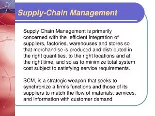
In this lecture, we conclude Chapter 6 on decision tree analysis and introduce Chapter 7 focusing on forecasting. We analyze a new product with uncertain demand, evaluating annual demand changes and their probabilities. We employ discount factors to calculate the Net Present Value (NPV) for various scenarios. Applications of decision trees for network design and logistics strategies are discussed, including warehousing decisions and transportation capacity portfolio management. Homework 2 is due tomorrow before 5:00 PM.

E N D
Supply Chain Management Lecture 10
Outline • Today • Finish Chapter 6 (Decision tree analysis) • Start chapter 7 • Tomorrow • Homework 2 due before 5:00pm • Next week • Chapter 7 (Forecasting)
Example: Decision Tree Analysis • New product with uncertain demand ($85 profit/unit) • Annual demand expected to go up by 20% with probability 0.6 • Annual demand expected to go down by 20% with probability 0.4 • Use discount factor k = 0.1
Example • Represent the tree, identifying all states as well as all transition probabilities Period 2 P = 120*85+(0.6*12240+0.4*8160)/1.1 = 19844 P = 12240 Period 1 D=144 0.6 Period 0 D=120 0.6 0.4 P = 8160 D=100 D=96 0.6 0.4 P = 100*85+(0.6*19844+0.4*13229)/1.1 = 24135 D=80 0.4 P = 5440 D=64 P = 80*85+(0.6*8160+0.4*5440)/1.1 = 13229
Example • Represent the tree, identifying all states as well as all transition probabilities Period 2 Period 1 D=144 0.6 Period 0 D=120 0.6 0.4 D=100 D=96 0.6 0.4 D=80 0.4 D=64 Calculate the NPV of each possible scenario separately
Period 2 Period 1 D=144 0.6 Period 0 D=120 0.6 0.4 D=100 D=96 0.6 0.4 D=80 0.4 D=64 Example • Represent the tree, identifying all states as well as all transition probabilities Calculate the NPV of each possible scenario separately
Decision Trees (Summary) • A decision tree is a graphic device used to evaluate decisions under uncertainty • Identify the duration of each period and the number of time periods T to be evaluated • Identify the factors associated with the uncertainty • Identify the representation of uncertainty • Identify the periodic discount rate k • Represent the tree, identifying all states and transition probabilities • Starting at period T, work back to period 0 identify the expected cash flows at each step • (Alternatively, calculate the NPV of each possible scenario separately)
Decision Trees • Using decision trees to evaluate network design decisions • Should the firm sign a long-term contract for warehousing space or get space from the spot market as needed • What should the firm’s mix of long-term and spot market be in the portfolio of transportation capacity • How much capacity should various facilities have? What fraction of this capacity should be flexible?
Example: Decision Tree Analysis • Three options for Trips Logistics • Get all warehousing space from the spot market as needed • Sign a three-year lease for a fixed amount of warehouse space and get additional requirements from the spot market • Sign a flexible lease with a minimum change that allows variable usage of warehouse space up to a limit with additional requirement from the spot market
Example: Decision Tree Analysis • Trips Logistics input data • Evaluate each option over a 3 year time horizon (1 period is 1 year) • Demand D may go up or down each year by 20% with probability 0.5 • Warehouse spot price p may go up or down by 10% with probability 0.5 • Discount rate k = 0.1
Period 2 D=144 p=$1.45 Period 1 D=144 p=$1.19 D=120 p=$1.32 D=96 p=$1.45 D=144 D=120 p=$0.97 p=$1. 08 D=96 p=$1.19 D=80 D=96 p=$1.32 p=$0.97 D=64 p=$1.45 D=80 p=$1.08 D=64 p=$1.19 D=64 p=$0.97 Example • Represent the tree, identifying all states 0.25 0.25 0.25 0.25 0.25 Period 0 0.25 D=100 0.25 p=$1.20 0.25
Example – Option 1 (Spot) Period 2 • Starting at period T, work back to period 0 identify the expected cash flows at each step • C(D = 144,000, p = 1.45, 2) = 144,000 x 1.45 = $208,800 • R(D = 144,000, p = 1.45, 2) = 144,000 x 1.22 = $175,680 • P(D = 144,000, p = 1.45, 2) = R – C = 175,680 – 208,800 = –$33,120 D=144 p=$1.45 D=144 p=$1.19 D=96 Cost p=$1.45 D=144 p=$0.97 Revenue D=96 p=$1.19 D=96 Profit p=$0.97 D=64 p=$1.45 D=64 p=$1.19 D=64 p=$0.97
Example – Option 1 (Spot) Period 2 • Starting at period T, work back to period 0 identify the expected cash flows at each step D=144 p=$1.45 D=144 p=$1.19 D=96 p=$1.45 D=144 p=$0.97 D=96 p=$1.19 D=96 p=$0.97 D=64 p=$1.45 D=64 p=$1.19 D=64 p=$0.97
Period 2 D=144 p=$1.45 Period 1 0.25 D=144 0.25 p=$1.19 D=120 0.25 D=96 p=$1.32 p=$1.45 0.25 D=96 p=$1.19 Example – Option 1 (Spot) • Starting at period T, work back to period 0 identify the expected cash flows at each step • EP(D = 120, p = 1.22, 1) = 0.25xP(D = 144, p = 1.45, 2) + 0.25xP(D = 144, p = 1.19, 2) + 0.25xP(D = 96 p = 1.45, 2) + 0.25xP(D = 96, p = 1.19, 2) = –$12,000 • PVEP(D = 120, p = 1.22, 1) = EP(D = 120, p = 1.22, 1)/(1+k) = –12,000/1.1 = –$10,909
Period 2 D=144 p=$1.45 Period 1 0.25 D=144 0.25 p=$1.19 D=120 0.25 D=96 p=$1.32 p=$1.45 0.25 D=96 p=$1.19 Example – Option 1 (Spot) • Starting at period T, work back to period 0 identify the expected cash flows at each step • P(D = 120, p = 1.32, 1) = R(D = 120, p = 1.22, 1) – C(D = 120, p = 1.32, 1) + PVEP(D = 120, p = 1.22, 1) = $146,400 - $158,400 + (–$10,909) = –$22,909
Period 2 D=144 p=$1.45 0.25 Period 1 D=144 0.25 p=$1.19 D=120 0.25 D=96 p=$1.32 p=$1.45 0.25 D=144 D=120 p=$0.97 p=$1. 08 D=96 p=$1.19 D=80 D=96 p=$0.97 p=$1.32 D=64 p=$1.45 D=80 D=64 p=$1.32 p=$1.19 D=64 p=$0.97 Example – Option 1 (Spot) • Starting at period T, work back to period 0 identify the expected cash flows at each step
Period 2 D=144 p=$1.45 Period 1 0.25 D=144 0.25 p=$1.19 D=120 0.25 D=96 p=$1.32 0.25 p=$1.45 0.25 D=144 Period 0 0.25 D=120 p=$0.97 p=$1. 08 D=100 D=96 0.25 p=$1.20 p=$1.19 D=80 D=96 p=$0.97 p=$1.32 D=64 0.25 p=$1.45 D=80 D=64 p=$1.32 p=$1.19 D=64 p=$0.97 Example – Option 1 (Spot) • Starting at period T, work back to period 0 identify the expected cash flows at each step NPV(Spot) = $5,471
Example: Decision Tree Analysis • Three options for Target.com • Get all warehousing space from the spot market as needed • Sign a three-year lease for a fixed amount of warehouse space and get additional requirements from the spot market • Get 100,000 sq ft. of warehouse space at $1 per square foot • Additional space purchased from spot market • Sign a flexible lease with a minimum change that allows variable usage of warehouse space up to a limit with additional requirement from the spot market
Example – Option 2 (Fixed lease) • Starting at period T, work back to period 0 identify the expected cash flows at each step Period 2 D=144 p=$1.45 Period 1 0.25 D=144 0.25 p=$1.19 D=120 0.25 D=96 p=$1.32 0.25 p=$1.45 0.25 D=144 Period 0 0.25 D=120 p=$0.97 p=$1. 08 D=100 D=96 0.25 p=$1.20 p=$1.19 D=80 D=96 p=$0.97 p=$1.32 D=64 0.25 p=$1.45 D=80 D=64 p=$1.32 p=$1.19 D=64 p=$0.97
Example – Option 2 (Fixed lease) • Starting at period T, work back to period 0 identify the expected cash flows at each step • P(D =, p =, 2) = R(D =, p =, 2) – C(D =, p =, 2) • P(D =, p =, 2) = Dx1.22 – (100,000x1.00 + Sxp) 8
Example – Option 2 (Fixed lease) • Starting at period T, work back to period 0 identify the expected cash flows at each step • P(D =, p =, 1) = R(D =, p =, 1) – C(D =, p =, 1) + PVEP(D =, p =, 1) • P(D =, p =, 1) = Dx1.22 – (100,000x1.00 + Sxp) + EP(D =, p =, 1)/(1+k)
Example – Option 2 (Fixed lease) • Starting at period T, work back to period 0 identify the expected cash flows at each step • P(D =, p =, 0) = R(D =, p =, 0) – C(D =, p =, 0) + PVEP(D =, p =, 0) • P(D =, p =, 0) = 100,000x1.22 – 100,000x1.00 + 16,364/1.1 NPV(Fixed lease) = $38,364
Example: Decision Tree Analysis • Three options for Target.com • Get all warehousing space from the spot market as needed • Sign a three-year lease for a fixed amount of warehouse space and get additional requirements from the spot market • Sign a flexible lease with a minimum change that allows variable usage of warehouse space up to a limit with additional requirement from the spot market • $10,000 upfront payment • Use anywhere between 60,000 and 100,000 sq ft. at $1 per sq ft. • Additional space purchased from spot market
Example – Option 3 (Flexible lease) • Flexible lease rules • Up-front payment of $10,000 • Flexibility of using between 60,000 and 100,000 sq.ft. at $1.00 per sq.ft. per year • Additional space requirements from spot market
Example – Option 3 (Flexible lease) • Starting at period T, work back to period 0 identify the expected cash flows at each step Period 2 D=144 p=$1.45 Period 1 0.25 D=144 0.25 p=$1.19 D=120 0.25 D=96 p=$1.32 0.25 p=$1.45 0.25 D=144 Period 0 0.25 D=120 p=$0.97 p=$1. 08 D=100 D=96 0.25 p=$1.20 p=$1.19 D=80 D=96 p=$0.97 p=$1.32 D=64 0.25 p=$1.45 D=80 D=64 p=$1.32 p=$1.19 D=64 p=$0.97
Example – Option 3 (Flexible lease) • Starting at period T, work back to period 0 identify the expected cash flows at each step • P(D =, p =, 2) = R(D =, p =, 2) – C(D =, p =, 2) • P(D =, p =, 2) = Dx1.22 – (Wx1.00 + Sxp)
Example – Option 3 (Flexible lease) • Starting at period T, work back to period 0 identify the expected cash flows at each step • P(D =, p =, 1) = R(D =, p =, 1) – C(D =, p =, 1) + PVEP(D =, p =, 1) • P(D =, p =, 1) = Dx1.22 – (Wx1.00 + Sxp) + EP(D =, p =, 1)/(1+k) 20,000 20,000
Example – Option 3 (Flexible lease) • Starting at period T, work back to period 0 identify the expected cash flows at each step • P(D =, p =, 0) = R(D =, p =, 0) – C(D =, p =, 0) + PVEP(D =, p =, 0) • P(D =, p =, 0) = 100,000x1.22 – 100,000x1.00 + 38,198/1.1 NPV(Flexible lease) = 56,725 – 10,000 = $46,725
From Design to Planning • Network design • C4 Designing Distribution Networks • C5 Network Design in the Supply Chain • C6 Network Design in an Uncertain Environment • Planning in a supply chain • C7 Demand Forecasting in a Supply Chain • C8 Aggregate Planning in a Supply Chain • C9 Planning Supply and Demand
Demand Forecasting • How does BMW know how many Mini Coopers it will sell in North America? • How many Prius cars should Toyota build to meet demand in the U.S. this year? Worldwide? • When is it time to tweak production, upward or downward, to reflect a change in the market? What factors influence customer demand?
Factors that Affect Forecasts • Past demand • Time of year/month/week • Planned advertising or marketing efforts • Planned price discounts • State of the economy • Market conditions • Actions competitors have taken
Example: Demand Forecast for Milk • A supermarket has experienced the following weekly demand (in gallons) over the last ten weeks • 109, 116, 108, 103, 97, 118, 120, 127, 114, and 122 What is a reasonable demand forecast for milk for the upcoming week? When could using average demand as a forecast lead to an inaccurate forecast? If demand turned out to be 125 what can you say about the demand forecast?
1) Characteristics of Forecasts • Forecasts are always wrong! • Forecasts should include an expected value and a measure of error (or demand uncertainty) • Forecast 1: sales are expected to range between 100 and 1,900 units • Forecast 2: sales are expected to range between 900 and 1,100 units
2) Characteristics of Forecasts • Long-term forecasts are less accurate than short-term forecasts • Less easy to consider other variables • Hard to include the effects of weather in a forecast • Forecast horizon is important, long-term forecast have larger standard deviation of error relative to the mean
3) Characteristics of Forecasts • Aggregate forecasts are more accurate than disaggregate forecasts
3) Characteristics of Forecasts • Aggregate forecasts are more accurate than disaggregate forecasts • They tend to have a smaller standard deviation of error relative to the mean Monthly sales SKU Monthly sales product line
4) Characteristics of Forecasts • Information gets distorted when moving away from the customer • Bullwhip effect
Characteristics of Forecasts • Forecasts are always wrong! • Long-term forecasts are less accurate than short-term forecasts • Aggregate forecasts are more accurate than disaggregate forecasts • Information gets distorted when moving away from the customer
Role of Forecasting Supplier Manufacturer Distributor Retailer Customer Push Push Push Pull Push Push Pull Push Pull Is demand forecasting more important for a push or pull system?
Types of Forecasts • Qualitative • Primarily subjective, rely on judgment and opinion • Time series • Use historical demand only • Causal • Use the relationship between demand and some other factor to develop forecast • Simulation • Imitate consumer choices that give rise to demand
Components of an Observation • Quarterly demand at Tahoe Salt Actual demand (D)
Components of an Observation • Quarterly demand at Tahoe Salt Level (L) and Trend (T)
Components of an Observation • Quarterly demand at Tahoe Salt Seasonality (S)
Components of an Observation Observed demand = Systematic component + Random component L Level (current deseasonalized demand) T Trend (growth or decline in demand) S Seasonality (predictable seasonal fluctuation)
Time Series Forecasting Forecast demand for the next four quarters.