Probability in Modeling
Probability in Modeling. D. E. Stevenson Shodor Education Foundation Steve@shodor.org. An Aside on Matlab. Population in Stella Revisited. Stella Model with Random Population Change. Pop(t+1) = Pop(t) average rate of change + random deviation [-6,6] rate Pop(t) 2 .

Probability in Modeling
E N D
Presentation Transcript
Probability in Modeling D. E. Stevenson Shodor Education Foundation Steve@shodor.org
Stella Model with Random Population Change Pop(t+1) = Pop(t)average rate of change + random deviation [-6,6] ratePop(t)2.
Diffusion Processes “Diffusion refers to the process by which molecules intermingle as a result of their kinetic energy of random motion. Molecules are in constant motion and make numerous collisions.” (edited version from hyperphysics.phy-astr.gsu.edu)
Modeling the Physics • Kinetic Energy is mv2/2. • Temperature T in K = E(mv2/3/k) k = 1.3810-23 joules/ K • Assume motion in all three dimensions.
Some Real Stuff • What does this all mean for a pile of sugar? • Mass of sucrose is 342 daltons. • Velocity in sucrose 81 m/sec. • Mean free path about 4.510-10 cm (durn rough estimate). • Mean time between collisions 5.610-10 sec.
Model=Random Walk • Let x(n) be the location of a particle at time t. x(0)=0 • The particle moves a fixed (unit) distance every time interval at a speed of ufor an effective length of u. • The probability that particle moves to the right is p and to the left q. • Time step directions are independent.
Final Location • Assume that the particles don’t transfer momentum. Consider the trajectory of a single particle. Assume p=q=1/2. • Where does the particle end up? • Matlab d1drwalk1.m d1drwalk2.m
Computing Ensemble Average • Let xi(n)the position of particle i attime n. • The rule is • So the average is
Finalizing • The average of the steps is zero if p=q. • Then the average location at time n is the same as that of n-1. • Recursively, then the average location is the same as the starting location…zero.
Computing Ensembles • Now let’s consider many particles, all starting at X(0)=0. Assume these do not collide with one another. All these particles together form an ensemble. • What can we say about the ensemble? d1drwalk4.m • But isn’t it zero? d1drwalk4bin.m
Ensemble Average • Here’s the uncertainty. We ran a small number of trials (M=100) for a short period of time (N=500 steps). • I need to consider • Is M big enough? • Is N big enough? • Ah, is the random sequence good enough? d1drwalk5.m
Summary • We have considered some of the history of probability in science as opposed to its use as a mathematical subject. • We considered very briefly the diffusion process and random walks as a implementation. • We saw that ensembles may or may not be well constructed by Matlab.
A little history • Jakob (Jacques) Bernoulli, Ars Conjectandi, 1713. • Thomas Bayes, Essay towards solving a problem in the doctrine of chances, 1764. • Pierre-Simon Laplace, Essai philosophique sur les probabilités, 1812. • George Boole, An investigation into the Laws of Thought, on Which are founded the Mathematical Theories of Logic and Probabilities, 1854.
More Modern… • Copenhagen Meeting, 1927. • William Feller, Introduction to Probability Theory and its Applications (1950-61). • Sir Harold Jefferys, Theory of Probability, 1939. • Samuel Karlin, A First Course in Stochastic Processes, 1969. A Second Course in Stochastic Processes, 1981. • Edwin T. James, Probability as Extended Logic, 1995 (bayes.wustl.edu)