Download
1 / 30
300 likes | 631 Views
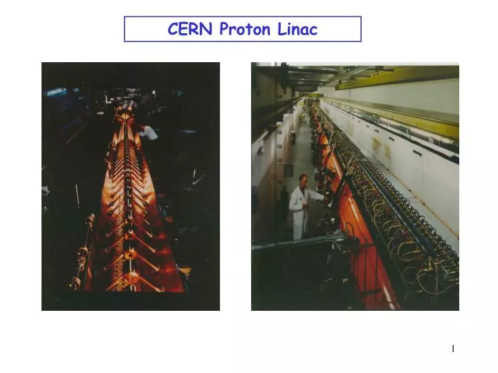
CERN Proton Linac. Multi-gaps Accelerating Structures: B- High Energy Electron Linac.

E N D
Multi-gaps Accelerating Structures:B- High Energy Electron Linac - When particles gets ultra-relativistic (v~c) the drift tubes become very long unless the operating frequency is increased. Late 40’s the development of radar led to high power transmitters (klystrons) at very high frequencies (3 GHz). - Next came the idea of suppressing the drift tubes using traveling waves. However to get a continuous acceleration the phase velocity of the wave needs to be adjusted to the particle velocity. solution: slow wave guide with irises iris loaded structure
Iris Loaded Structure for Electron Linac Photo of a CGR-MeV structure 4.5 m long copper structure, equipped with matched input and output couplers. Cells are low temperature brazed and a stainless steel envelope ensures proper vacuum.
Other types of S.W. Multi-cells Cavities nose cone side coupled
Energy-phase Equations - Rate of energy gain for the synchronous particle: - Rate of energy gain for a non-synchronous particle, expressed in reduced variables, and : - Rate of change of the phase with respect to the synchronous one: Since:
Energy-phase Oscillations one gets: Combining the two first order equations into a second order one: with Stable harmonic oscillations imply: hence: And since acceleration also means: One finally gets the results:
The Capture Problem • Previous results show that at ultra-relativistic energies ( >> 1) the longitudinal motion is frozen. Since this is rapidly the case for electrons, all traveling wave structures can be made identical (phase velocity=c). • Hence the question is: can we capture low kinetic electrons energies ( < 1), as they come out from a gun, using an iris loaded structure matched to c ? e- v=c 0 < 1 gun structure The electron entering the structure, with velocity v < c, is not synchronous with the wave. The path difference, after a time dt, between the wave and the particle is: Since: one gets: and
The Capture Problem (2) From Newton-Lorentz: Introducing a suitable variable: the equation becomes: Using Integrating from t0to t (from =0 to =1) Capture condition
Improved Capture With Pre-buncher A long bunch coming from the gun enters an RF cavity; the reference particle is the one which has no velocity change. The others get accelerated or decelerated. After a distance L bunch gets shorter while energies are spread: bunching effect. This short bunch can now be captured more efficiently by a TW structure (v=c).
Improved Capture With Pre-buncher (2) The bunching effect is a space modulation that results from a velocity modulation and is similar to the phase stability phenomenon. Let’s look at particles in the vicinity of the reference one and use a classical approach. Energy gain as a function of cavity crossing time: Perfect linear bunching will occur after a time delay , corresponding to a distance L, when the path difference is compensated between a particle and the reference one: (assuming the reference particle enters the cavity at time t=0) Since L = vone gets:
The Synchrotron (Mac Millan, Veksler, 1945) The synchrotron is a synchronous accelerator since there is a synchronous RF phase for which the energy gain fits the increase of the magnetic field at each turn. That implies the following operating conditions: Energy gain per turn Synchronous particle RF synchronism Constant orbit Variable magnetic field If v = c,wrhencewRFremain constant (ultra-relativistic e- )
The Synchrotron (2) Energy ramping is simply obtained by varying the B field: Since: • The number of stable synchronous particles is equal to the harmonic number h. They are equally spaced along the circumference. • Each synchronous particle satifies the relation p=eB. They have the nominal energy and follow the nominal trajectory.
The Synchrotron (3) During the energy ramping, the RF frequency increases to follow the increase of the revolution frequency : hence : Since , the RF frequency must follow the variation of the B field with the law : which asymptotically tends towards when B becomes large compare to (m0c2 / 2pr) which corresponds to v c (pc >> m0c2 ). In practice the B field can follow the law:
Zero gradient synchrotron retour
Alternating gradient synchrotron Non parallel pole faces shows a field gradient. If focusing in one plane, defocusing in the other one. Alternating focusing and defocusing magnets can lead to global focusing.
Separated functions synchrotron Quadrupole + Dipole = FODO system retour Super Protons Synchrotron at CERN
Single Gap Types Cavities Pill-box variants noses disks Coaxial cavity Type /4
Ferrite Loaded Cavities • Ferrite toroids are placed around the beam tube which allow to reach lower frequencies at reasonable size. • Polarizing the ferrites will change the resonant frequency, hence satisfying energy ramping in protons and ions synchrotrons.
Dispersion Effects in a Synchrotron cavity If a particle is slightly shifted in momentum it will have a different orbit: E Circumference 2R This is the “momentum compaction” generated by the bending field. E+E If the particle is shifted in momentum it will have also a different velocity. As a result of both effects the revolution frequency changes: p=particle momentum R=synchrotron physical radius fr=revolution frequency
Dispersion Effects in a Synchrotron (2) x d The elementary path difference from the two orbits is: leading to the total change in the circumference: < >mmeans that the average is considered over the bending magnet only Since: we get:
Dispersion Effects in a Synchrotron (3) =0 at the transition energy
Phase Stability in a Synchrotron From the definition of it is clear that below transition an increase in energy is followed by a higher revolution frequency (increase in velocity dominates) while the reverse occurs above transition (v c and longer path) where the momentum compaction (generally > 0) dominates. Stable synchr. Particle for <0 > 0
Longitudinal Dynamics It is also often called “ synchrotron motion”. The RF acceleration process clearly emphasizes two coupled variables, the energy gained by the particle and the RF phase experienced by the same particle. Since there is a well defined synchronous particle which has always the same phase s, and the nominal energy Es, it is sufficient to followother particles with respect to that particle. So let’s introduce the following reduced variables: revolution frequency : fr = fr – frs particle RF phase : = - s particle momentum : p = p - ps particle energy : E = E – Es azimuth angle : = - s
First Energy-Phase Equation R For a given particle with respect to the reference one: Since: and one gets:
Second Energy-Phase Equation The rate of energy gained by a particle is: The rate of relative energy gain with respect to the reference particle is then: Expanding the left hand side to first order: leads to the second energy-phase equation:
Equations of Longitudinal Motion deriving and combining This second order equation is non linear. Moreover the parameters within the bracket are in general slowly varying with time…………………
Hamiltonian of Longitudinal Motion Introducing a new convenient variable, W, leads to the 1th order equations: These equations of motion derive from a hamiltonian H(,W,t):
Small Amplitude Oscillations Let’s assume constant parameters Rs,ps,s and : with Consider now small phase deviations from the reference particle: (for small ) and the corresponding linearized motion reduces to a harmonic oscillation: stable for and s real < tr > 0 0 < s < /2 sins > 0 > tr < 0 /2 < s < sins > 0