A Novel Wave-Propagation Approach For Fully Conservative Eulerian Multi-Material Simulation
260 likes | 379 Views
This presentation explores a novel approach to wave propagation in fully conservative Eulerian multi-material simulations, targeting high-speed solid-solid and solid-fluid interactions. We discuss challenges with traditional level set methods, emphasizing spatial accuracy and conservation issues. The talk introduces Cartesian cut-cell meshes, highlights existing techniques addressing small cell problems, and details the extension of LeVeque and Shyue's front-tracking method to ensure full conservativity across multiple materials. We present examples in both 1D and 2D, concluding with our future research directions.

A Novel Wave-Propagation Approach For Fully Conservative Eulerian Multi-Material Simulation
E N D
Presentation Transcript
A Novel Wave-Propagation Approach For Fully Conservative Eulerian Multi-Material Simulation K. Nordin-Bates With thanks to AWE for funding! Lab. for Scientific Computing, Cavendish Lab., University of Cambridge
Outline • Motivation • Brief introduction to Cartesian cut-cell approaches • LeVeque & Shyue’s Front-tracking Wave Propagation Method • Extension to a fully conservative multi-material algorithm • Examples in 1D – Fluid and strength. • Extension to two dimensions • Fluid examples in 2D • Conclusions and Next steps
Motivation • We’re interested in simulating high-speed solid-solid and solid-fluid interaction involving large deformations. • Our current approach employs a level set method for representation of interfaces coupled with a deformation gradient formulation for elastic-plastic strength. • This appears to give reasonable results for many situations. • However, there are some drawbacks to the approach: • Spatial accuracy at the boundary is limited since the precise location of the interface within cells is lost. • The method is not mass or energy conservative (even if the level set is updated in a conservative manner). • Problems may occur at concave interfaces since single ghost cells attempt to satisfy multiple boundary conditions.
Cut-Cell Meshes and their Challenges • We are therefore also investigating the use of Cartesian cut-cell meshes for the simulation of such configurations. • In such methods the material interface (or boundary) cuts through a regular underlying mesh, resulting in a single layer of irregular cells adjacent to the interface. • The primary challenge associated with solving hyperbolic systems on such meshes using standard explicit methods is a time-step limit of the order of the cell volume (and these volumes may be arbitrarily small)
Some Existing Cut-Cell Approaches • Various approaches have been developed to overcome this ‘small cell problem’: • Cell merging: e.g. Clarke, Salas & Hassan 1986 • Flux redistribution / stabilisation schemes: e.g. Colella et al. 2006 • Rotated Grid / h-Box scheme: Berger et al. 2003 • We ideally want a method that : • Is stable at a time-step determined by regular cells. • Copes with moving interfaces. • Can handle arbitrary no. of materials and interfaces in a cell • Works in multi-dimensions and preserves symmetry
Leveque & Shyue Front Tracking Method • LeVeque & Shyue 1996 introduced a method for the simulation of problems in which an embedded front is tracked explicitly in parallel with a solution on a regular mesh • They proposed a ‘large time-step’ scheme in which the propagation of waves from each interface into multiple target volumes is considered. • However, this scheme as originally constructed is not fully conservative for multi-material simulation, since waves from cell interfaces cross the embedded interface. (Diagram taken from Leveque & Shyue 1996)
1D Wave Propagation Method • We begin by considering the original scheme of L&S in 1D for the system of conservation laws • At each interface we compute a Roe-type linearized Riemann Problem solution with wave speeds and state jumps across these - we have , and • A conservative first order explicit update for the solution in cell is then given by
Front Tracking Version of WPM • This approach was extended to incorporate front-tracking. Suppose we have a point defining the front of interest laying in cell . • We store states in each portion of the cell, and can hence compute a RP between these, which gives waves propagating into each material as well as the speed of the front. • Note that waves from the front cross neighbouring cell interfaces, and vice-versa. • To obtain a stable update for the same time-step as the regular cells, we add the contributions of these waves to the multiple cells that they cross.
Fully Conservative Multi-Material Extension • Through the use of a multi-material RP solver at the tracked front, the basic mechanism may be extended in a natural way to cope with multiple materials. • (The details of multi-material RP solvers are skipped here.) • To make the approach conservative within each material, we need to avoid waves crossing the embedded interface: • We achieve this here by identifying the arrival time of the incoming wave with the interface and posing an intermediate RP at this point. • This is repeated for each wave arriving at the interface
Some comments • Won’t state full update formula here(!), but is built up from contribution due to waves. • Interacting waves impart a “full cell contribution” to the update of the relevant cut-cell states. • For example, in the example update to the right, the fastestwave from the interface contributes to the update of • …while the left-going wave from the first interaction contributes for the wave arrival timeand the corresponding RP solution • Note that if the interface crosses into a neighbouring cell within a time-step, we need to consider incoming waves from the edges of this cell too. • Also, note that if we’re only simulating a single material, the Roe-type Riemann solver used for the regular cell interfaces is insufficient for producing an interface solution.
Fully Conservative Multi-Material Extension • The algorithm for updating becomes: • Compute RP solutions at t=0 for all regular and embedded interfaces. • Initialize interface-adjacent states to initial cell values for all mixed cells. • While there are waves interacting with an embedded interface: • Identify next wave to interact • Update interface adjacent states to star states of most recent interface RP • Add incoming wave jump to relevant state, e.g. := • Solve resultant intermediate RP between , and store. • Update solution using contributions from all waves from all RPs.
One-Dimensional Fluid Examples • First examples demonstrate the scheme applied to single material Euler equations with ideal gas EoS. • (i.e. this essentially uses the scheme in a fully-conservative contact-front-tracking mode) • We consider a Sod-type problem with initial condition given by and with constant adiabatic constant . • Simulations are run at , with to , and we consider initial interface positions at and as illustrated below. • The exact solution consists of a right-travelling shock and contact and left-travelling rarefaction:
One-Dimensional Fluid Example: Single Material • Snapshots of the results of both tests at : • Total mass conservation errors are of the order of machine accuracy:
Second Order Extension • The method is extended to second order accuracy in much the same way as the original WPM, with linear correction profiles added to each wave. • Taylor series analysis gives a correction • Modification is required on cut-cells. • We apply limiting to wave strengths toensure monotonicity. • Plot shows equivalent simulation to before, with 2nd order solver. • Conservation unaffected by correction.
One dimensional Fluid Example: Multi-material • Now extend previous test to multi-material ideal gas case, with , • Density snapshots at , run with in case with barrier at : • Relative mass error <1e15 for each component throughout in both cases Barrier x=0 Barrier x=1
One-Dimensional Strength Examples • Mass conservation: • Momentum conservation: • Energy conservation: • Total deformation: • Plastic deformation: • Work hardening:
Strength test comments • Ignoring plastic source terms for now, this is a hyperbolic system with 22 waves (of which 16 are linearly degenerate of speed and 6 genuinely non-linear) • One longitudinal wave (p-wave) and 2 shearwaves (s-waves) in each direction. • Disclaimer: the linearized approximate Riemann solver used here does not satisfy Roe criterion, hence WPM is not conservative (even without interfaces!) • But, want to demonstrate stability of approach for systems involving more complex eigenstructures.
One-Dimensional Strength Examples • We consider a purely elastic 1D impact problem in which pre-deformed copper and steel plates collide. • The problem is contrived such that the solution demonstrates a full family of waves • Initial conditions and material models are taken from first test-case of Barton & Drikakis2010 • The problem is solved on a domain of length with regular cell size to time • The initial interface is located at and propagates through approx. 25 cells during the simulation. • ‘Stick’ interface conditions are used.
Conservation for non-Roe-type solvers • We can also consider how the approach may be made conservative for approximate Riemann solvers that do not satisfy the Roe criterion. • This requires considering the effect of the waves on the interface flux (rather than using them directly in the update). • For example, here we assemble a left interface flux • We may use these in a standard flux update. • This modification has an additional computational cost compared with the WPM approach, as the flux function must be evaluated multiple times per interface. • Results for fluid problems are qualitatively identical to WPM, but with exact conservation.
2D Unsplit Wave Propagation Method • For now, we consider the extension of the method to 2D for a single material with rigid interfaces. • Consider a single regular cell interface in 2D: solving the Riemann problem normal to the interface gives a family of waves emitted from the interface: • Dimensionally unsplit WPM accounts for tangential propagation of these waves by decomposing each of them using the tangential flux eigenstructure:
2D Unsplit WPM with Interfaces • Essentially, we obtain a collection of parallelograms and update the solution based on the wave jumps and the cells overlapped by the parallelograms. • We can do the same at interior interfaces (using a multi-material RP solver for the normal direction)
2D Wave-Interface Interaction • As in 1D, waves from regular interfaces may cross the interior interface within a time-step. • This impact is determined by simple geometric test and an ‘impact area’ identified. • Impact time may be taken as the average (i.e. time at which centre is hit). • At this point, we pose a new interface RP (for entire interior interface) and propagate resultant waves.
2D Results • We demonstrate the method in action with a very simple example problem of a Mach 1.49 shock in air hitting a ‘double’ wedge at 55°.
Conclusions & Next Steps • Demonstrated a novel multi-interaction version of the Wave Propagation Method incorporating material interface tracking giving mass conservation in each material individually (to machine accuracy) in 1D. • The approach has been extended to 2D and again shows mass conservation for a single material with static embedded boundaries. • Additionally have preliminary results with moving interfaces in 2D (not presented) – not yet fully conservative. • Further research: • Rigorous comparison of accuracy and expense as compared to alternative cut-cell approaches. • Investigate use of approximate multi-material Riemann solvers. • Further investigating of moving boundary conservation in 2D. • 3D!
Constant Interface Velocity Modification • While the original approach is functional in 1D,varyingof interface velocity within a time-step is impractical inmulti-dimensions. • We therefore propose a modification in which the interface velocity remains constant within each time-step. • This velocity is decided by the RP solution at the beginningof the time-step, which is solved in the normal way. • Intermediate interactions then present a modified interface problem, in which we no longer require pressures to match at the interface, but instead require it to match the prescribed velocity.