2D Output Primitives
Point plotting. A coordinate position in an application program corresponds to a pixel (picture element) position on an output deviceTypically, a memory position in a frame buffer (display memory) corresponds to a specific display position. Points (pixels). The size of a display point (pixel) is a


2D Output Primitives
E N D
Presentation Transcript
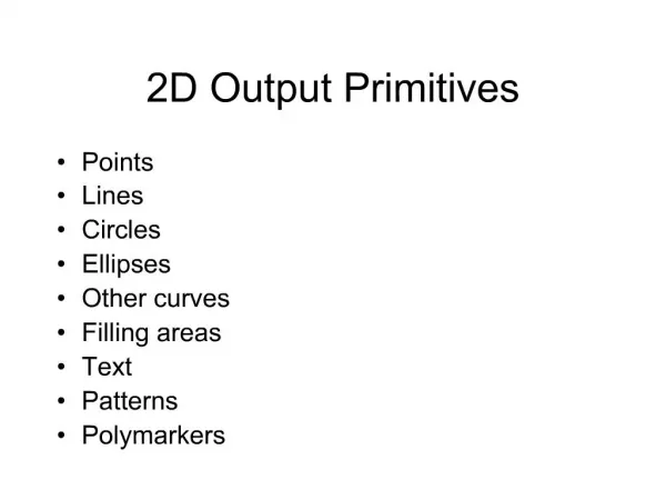
1. 2D Output Primitives Points
Lines
Circles
Ellipses
Other curves
Filling areas
Text
Patterns
Polymarkers
2. Point plotting A coordinate position in an application program corresponds to a pixel (picture element) position on an output device
Typically, a memory position in a frame buffer (display memory) corresponds to a specific display position
3. Points (pixels) The size of a display point (pixel) is a function of the diameter of the electron beam (if CRT) and the size of the phosphor spot on the display
Too small points => a grainy image
Too large points => a fuzzy image
The minimal functionality required to perform computer graphics:
setPixel(x, y, intensity)
intensity = getPixel(x, y)
4. Coordinate system
5. Coordinate pixels
6. Line plotting Given the two endpoints, line plotting means calculating intermediate pixel positions (scan conversion)
Requirements on a good line plotter:
Straight line
Ending correctly
Constant thickness
Thickness independent of length and direction
Fast drawing
7. Incremental methods Normally, incremental methods are used (point-by-point plotting)
Most usual are DDA methods (Digital Differential Analyzer), parametric
Lines (curves) are generated using the differential equation of the lines (curves)
For lines: y� = ?y/?x (constant)
where y = m.x + b (line equation) and
m = ?y/?x (line slope)
8. Technique Increment x and y by small steps proportional to the first derivatives of x and y, respectively
For an ideal display: increment x and y by ??x and ??y, ? �small�, from one endpoint position to the other
In practise: only integer coordinate positions are available on a device=> rounding to nearest integer position in each step necessary
Choose the increments ??x and ??y = 1 !
9. Line drawing algorithms Symmetric DDA
choose ? so that ?=2-n and 2n-1=max(?x,?y)<2n
Simple DDA
choose ?=1/max(?x,?y), i.e. unity steps in one direction
Bresenham�s algorithm
with an error term and unity steps in one direction
10. Example Symmetric DDA Endpoints (0,0) and (12,10)
?x =12, ?y=10, 2n-1=max(12,10)<2n
23=max(12,10)<24, i.e. n=4 and ?=1/16
Use ??x=12.1/16=3/4 and ??y= =10.1/16= 5/8 as increments in each step
Initiate with fraction part=0.5 (cp. rounding to nearest integer) and start in endpoint (0,0)
Results in 15 different points out of 17 generated in total
11. Example Simple DDA Endpoints (0,0) and (12,10)
?x =12, ?y=10, ?=1/max(?x,?y)
?=1/max(12,10)=1/12
Use ??x=12.1/12=1 (unity step!) and ??y= =10.1/12= 5/6 as increments in each step
Initiate with fraction part=0.5 (cp. rounding to nearest integer) and start in endpoint (0,0)
Results in 13 different points out of 13 generated in total
12. Plotted line Line with endpoints in (0,0) and (12,10) plotted with Symmetric DDA in the first diagram and Simple DDA and Bresenham in the second
13. Bresenham�s algorithm 1 A unit step is incremented in one direction - the direction with the biggest slope m. If -1=m=1 then unit steps in x else unit steps in y.
The other coordinate is changed depending on an error term e, which will be influenced by the algorithm
The error term e is defined by the distance between the exact line and a generated pixel position (see figure)
14. Error term
15. Bresenham�s algorithm 2 In each step m=?y/?x is added to e.
Before this is done, the sign of e decides whether the coordinate with the smallest slope is changed or not (always unit steps in the other coordinate)
Initiating e=?y/?x-0.5 gives (assume biggest slope in x):
e=0 => the exact line is above the current pixel, i.e. y is incremented and e is decremented by one
e<0 => the exact line is below the current pixel, i.e. y is not changed
Using integers only, if e is multiplied by 2?x => no divisions and only multiplications by 2
16. The algorithm Again, assume biggest slope in x and 0=m=1
Initiate e := 2?y - ?x
if e=0 then e:= e+(2?y - 2?x), xk+1 := xk+1, yk+1 := yk +1
if e<0 then e:= e + 2?y, xk+1 := xk+1
17. Example Bresenham Endpoints (0,0) and (12,10)
?x =12, ?y=10 => 0=m=1, i.e. unit steps in x (biggest slope)
=> 2?y = 20, 2?y-2?x = -4
Initiate error term e = 2?y-?x = 8
In each step (always incr x):
if e=0 then e:=e+(2?y-2?x)= e - 4 and incr y
if e<0 then e:=e+2?y= e + 20
Results in 13 different points out of 13 generated in total
18. Circle generating methods In general, assume circle midpoint in origin
If not, only a simple translation is required
f(x,y) = x2 + y2 - r2 = 0 (circle equation)
DDA-technique
Direct from the equation
Polar coordinates
Bresenham
19. DDA-technique First derivative of the equation:
2x + 2y . y� = 0 <=> y� = -x/y
If 2n-1 = r < 2n => choose ? = 2-n
xk+1 := xk + ? . yk
yk+1 := yk - ? . xk
20. Direct from the equation y2 = r2 - x2
In the sector from 90� to 45�, take small steps in x from 0 to r/sqrt(2) and cal-culate y=sqrt(r2 - x2) for each x
21. Using polar coordinates x = r . cos ?
y = r . sin ?
From 0 to ?/4 (45�), take small steps in ? and calculate x and y for each ?
22. Symmetry of a circle Calculation of a circle point (x,y) in one octant yields the circle points for the other seven octants
23. Intro to Bresenham The best approximation will be described if the pixels choosen are those closest to the true circle. If plotting from 90� to 45� the next pixel to be plotted is either given by
a) increment x by one
or
b) increment x by one and decrement y by one
A method which is only using integers, integer additions and multiplications by 2 and 4 (cp binary shifts) is described by Bresenham
24. Deriving Bresenham
25. Bresenham continued A decision (error) variable di is then defined:
di = D(Si) + D(Ti)
The initial value on this variable can be derived as:
d1 = 3 - 2r, where x0= 0 and yo= r
26. Bresenham continued The sign of the decision variable will then decide how to continue:
if di<0 then
xi:=xi-1 + 1
di+1:=di + 4xi-1 +6
else (if di=0)
xi:=xi-1 +1
yi:=yi-1 - 1
di+1:=di + 4(xi-1 - yi-1) + 10
27. Ellipse properties Given two fixed positions F1 and F2, the sum of the two distances from these points to any point P on the ellipse (d1+d2) is constant.
28. Ellipse Equation With the major and minor axes aligned with the coordinate axes the ellipse is said to be in standard position:
29. One approach Take small steps in x from xc to xc+rx and calculate y:
30. Symmetry can be used Only one quadrant needs to be calculated since symmetry gives the three other quadrants
31. General curves A direct method:
Given a general curve y = f(x), take small steps in x and calculate y=f(x) for each x.