Download
1 / 38
380 likes | 536 Views
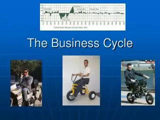
The business cycle. “A wavelike movement in the overall level of business activity”. The Business Cycle. Real GDP. Time. The term business cycle is used to describe observed fluctuations in key macroeconomic measures such as real GDP, personal income, profits, or employment.

E N D
The business cycle “A wavelike movement in the overall level of business activity”
The Business Cycle Real GDP Time • The term business cycle is used to describe observed fluctuations in key macroeconomic measures such as real GDP, personal income, profits, or employment. • A full cycle consists of an expansion and a contraction (or recession). • Business cycles are recurring phenomena; however, they are irregularly recurring.
The Burns and Mitchell (NBER) definition1 Business cycles are a type of fluctuation found in aggregate economic activity. . . . [A] cycle consists of expansions occurring at about the same time in many activities, followed by similarly general recessions, contractions, and revival which merge into the expansion phase of the next cycle; this sequence of change is recurrent but not periodic; in duration cycles vary from one year to 10 to 12 years. 1Burns, A. and Mitchell, W. Measuring Business Cycles. New York: National Bureau of economic Research, 1947, p. 3
2phases of the 1954-58 cycle Peak Real GDP Trough Trough Trend line contraction expansion Year/Month May ‘54 Aug. ‘57 Apr. ‘58 1Expansion was at 64 months through August, 1996. The NBER could date the peak retroactively, however.
Dating business cycles To date business cycle peaks and troughs, economists at the NBER look for well-defined turning points in key “coincident” indicators such as industrial production or nonfarm payrolls
Peak Trough www.bls.gov
A “full” business cycle consists of two “half-cycles”—an expansion is one half-cycle and the (chronologically) adjacent contraction is the other half cycle. The table on the following slide gives the record of cyclesin the U.S. since 1919, as dated by the NBER
Duration and Depth of Selected Business Cycles Contractions Source: Zarnowitz (1985), and Economagic.com 1The dates are 1923.2 to 1924.3; 1948.4 to 1949.4; 1953.3 to 1954.2; 1957.3 to 1958.2; 1973.4 to 1975.1; and 1981.3 to 1982.2. 2The dates are 1926.4 to 1927.4; 1960.2 to 1961.1; 1969.4 to 1970.4; and 1980.1 to 1980.3
Performance of GDP Components, 2007-IV to 2008-III. Source: Bureau of Economic Analysis
The “typical” business cycle Peak Economic Activity Trough Trough Stage I Stage II Stage III 1 year 2 years 1 year
Percent Change in Components of GDP Over the Business Cycle 1Based on the 1957-58, 1960-61, 1973-75, 1980, and 1981-82 recessions. Source: Oyen (1991).
Percent Change in Components of GDP Over the Business Cycle (Part 2) Source: Oyen (1991). 1Based on the 1957-58, 1960-61, 1973-75, 1980, and 1981-82 recessions. 2Excludes transfer payments
Aggregate Supply Aggregate supply: The relationship between the quantity of real GDP supplied and the price level when all other influences on production plans remain the same.
Aggregate Supply Basics • The quantity of real GDP supplied (Y) depends on: • The quantity of labor employed • The quantities of capital (including human capital) and the technologies they embody • The quantities of land and natural resources used • The amount of entrepreneurial talent available.
Change in the quantity of real GDP (Y) supplied Price level (GDP deflator) Potential GDP AS As price level increase, AS increases 110 As price level increase, AS increases 0 10.0 Real GDP (trillions of 1996 dollars)
As we move along AS, all other influences on productions plans remain constant (aside from the price level). • These influences include: • The money wage rate • The money prices of other resources
The Labor Market • Let • LS denote the supply of labor, which is presumed to be a positive function of the real wage, where the real wage is equal to the nominal wage divided by the price level (w/p). • LD denote the demand for labor, which is presumed to be a negative (or inverse) function of the real wage (w/p). As the real wage increases, the opportunity cost of leisure rises as well. Hence, people substitute work for leisure.
Diminishing Returns w/p I couldn’t afford to pay more than $15.25 for the second worker Plato’s LD $17.50 $15.25 0 1 2 Number of workers
The Labor Market Excess Supplyfor Labor LS $20 B A 15 E Real Hourly Wage = w/p H J 10 LD Excess Demandfor Labor 0 100 million = Full Employment Number of Workers
Potential GDP Corresponds to Labor Market Equilibrium Price level (GDP deflator) Potential GDP $10 trillion of real GDP can be produced when the economy is at full employment Note that potential GDP does not change when the price level changes 0 10.0 Real GDP (trillions of 1996 dollars)
Why is AS upward-sloping? Holding the nominal wage (w) constant, the real wage (w/p) decreases when the price level increases. This induces firms to hire more workers. Real GDP expands
Changes of Aggregate Supply • Aggregate supply can change (shift) due to • A change in the money wage • A change in the money prices of other productive resources • A change in potential GDP
Shifts of AS Price level (GDP deflator) Potential GDP • AS1 to AS0 • Falling wages or benefits costs. • Falling prices of other inputs (e.g., diesel fuel, rubber, copper, wood). AS1 AS0 110 0 10.0 Real GDP (trillions of 1996 dollars)
Potential GDP can change too Price level (GDP deflator) • Potential GDP can rise as a result of • Growth of the labor force • Capital accumulation including human capital • Improved technology Potential GDP 0 10.0 11.0 Real GDP (trillions of 1996 dollars)
The aggregate demand (AD) curve Price level (GDP deflator) The AD curve shows what spending units plan to spend at various price levels, holding all other influences on buying plans constant. AD 0 Real GDP (trillions of 1996 dollars)
Why is the AD curve downward-sloping? Price level (GDP deflator) • Change in the real interest rate • Change in the relative prices of exports and imports • Change in the buying power of money A 120 B 110 AD 0 Y1 Y2 Real GDP (trillions of 1996 dollars)
Changes (shifts) of (AD) curve Price level (GDP deflator) • AD0to AD1 is an increase in AD • AD0 to AD2 is a decrease in AD AD1 AD0 AD2 0 Real GDP (trillions of 1996 dollars)
What could cause AD to shift? • ADwill increase if: • Expected future income, profits, or inflation increase. • Government units or the Federal Reserve take steps to stimulate planned spending. • The exchange rate falls or the global economy expands
The Aggregate demand (AD Multiplier) Price level (GDP deflator) Increase in investment induces increase in C via the effect on income 110 AD1 AD0 +I Increase in I AD0 Induced increase in C 0 10.0 10.4 11.0 Real GDP (trillions of 1996 dollars)
The Aggregate Demand (AD) Fluctuations A business cycle might be explained strictly on the basis of fluctuations of AD. The next 2 slides show how investment fluctuations can produce a business cycle.
An aggregate demand (AD) cycle Price level Price level Potential GDP Potential GDP AS AS C C 115 115 D B E A AD2 AD2 105 105 AD3 AD1 AD4 AD0 0 0 9.5 10.0 10.5 9.5 10.0 10.5 RealGDP RealGDP Expansion Contraction
Real GDP Peak C 10.5 B D 10.0 A E 9.5 Full employment Trough Trough 5 2 3 4 1 Year
Stagflation is a combination of recession (falling real GDP) and inflation. Now we will show how stagflation could be produced by a supply shock
Price per barrel of 320 crude oil Source: Petroleum Economist
Stagflation due to oil price shock Price Level AS0 AS1 115 110 AD 0 9.75 10.0 Real GDP