Download
1 / 14
140 likes | 298 Views
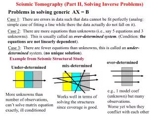
Seismic Tomography (Part II, Solving Inverse Problems). mix-determined. over-determined. Under-determined. e.g., 1 model coef (unknown) but many observations. Worse yet when they conflict with each other. Works well in terms of solving the structures since coverage is good.

E N D
Seismic Tomography (Part II, Solving Inverse Problems) mix-determined over-determined Under-determined e.g., 1 model coef (unknown) but many observations. Worse yet when they conflict with each other Works well in terms of solving the structures since coverage is good. More unknowns than number of observations, can’t solve matrix equation exactly, ill conditioned Problems in solving generic AX = B Case 1: There are errors in data such that data cannot be fit perfectly (analog: simple case of fitting a line while there the data actually do not fall on it). Case 2: There are more equations than unknowns (i.e., say 5 equations and 3 unknowns). This is usually called an over-determined system. (Condition: the equations are not linearly dependent). Case 3: There are fewer equations than unknowns, this is called an under-determined system. (no unique solution). Example from Seismic Structural Study
Tradeoff curves optimal Small damping large damping 2 2 1 3 1 3 Solution norm Fit to the data Damping factor Model size variation The sum of the squared values of elements of X (norm of X) goes to 0 since when we increase m, ATA matrix effectively becomes diagonal (with a very large number on the diagonal), naturally, X ----> 0 as aii ----> infinity.
Processes in seismic inversions in general Liu & Gu, Tectonophys, 2012
Simple Inverse Solver for Simple Problems Cramer’s rule: Suppose Consider determinant Now multiply D by x (consider some x value), by a property of the determinants, multiplication by a constant x = multiplication of a given column by x. Property 2: adding a constant times a column to a given column does not change determinant,
Then, follow same procedure, if D !=0, d != 0, Something good about Cramer’s Rule: It is simpler to understand It can easily extract one solution element, say x, without having to solve simultaneously for y and z. The so called “D” matrix can really be some A matrix multiplied by its transpose, i.e., D=ATA, in other words, this is equally applicable to least-squares problem.
Common matrix factorization methods Other solvers: (1) Gaussian Elimination and Backsubstitution: (2) LU Decomposition: L=lower triangular U=upper triangular Key: write A = L * U So in a 4 x 4, Advantage: can use Gauss Jordan Elimination on triangular matrices!
(3) Singular value decomposition (SVD): useful to deal with set of equations that are either singular or close to singular, where LU and Gaussian Elimination fail to get an answer for. Ideal for solving least-squares problems. Express A in the following form: U and V are orthogonal matrices (meaning each row/column vector is orthogonal). If A is square matrix, say 3 x 3, then U V and W are all 3 x 3 matrices. orthogonal matrices-Inverse=Transpose. So U and V are no problems and inverse of W is just 1/W, A-1 = V * [diag(1/wj)]*UT The diagonal elements of W are singular values, the larger, the more important for the large-scale properties of the matrix. So naturally, damping (smoothing) can be done by selectively throw out smaller singular values.
Model prediction A*X (removing smallest SV) Model prediction A*X (removing largest SV) We can see that a large change (poor fit) happens if we remove the largest SV, the change is minor if we remove the smallest SV.
Solution vector X[] elements Black --- removing none Red ---- keep 5 largest SV Green --- Keep 4 largest SV Generally, we see that the solution size decreased, SORT of similar to the damping (regularization) process in our lab 9, but SVD approach is not as predictable as damping. It really depends on the solution vector X and nature of A. The solutions can change pretty dramatically (even though fitting of the data vector doesn’t) by removing singular values. Imagine this operation of removal as changing (or zeroing out) some equations in our equation set.
2D Image compression: use small number of SV to recover the original image Keep all Keep 5 largest Keep 10 largest Keep 80 largest Keep 30 largest Keep 60 largest
Example of 2D SVD Noise Reduction South American Subduction System (the subducting slab is depressing the phase boundary near the base of the upper mantle) Cocos Plate South American Plate Nazca Plate 410 660 Courtesy of Sean Contenti
Result using all 26 Eigenvalues Pretty noisy with small-scale high amplitudes, both vertical and horizontal structures are visible.
Result using 10 largest Eigenvalues Some of the higher frequency components are removed from the system. Image appears more linear.
Retaining 7 largest eigenvalues Retaining 5 largest eigenvalues