Modeling and Performance Evaluation of Computer Systems
1.03k likes | 1.35k Views
Modeling and Performance Evaluation of Computer Systems. Chapter 3 Quantifying Performance Models. Performance by Design: Computer Capacity Planning by Example. Daniel A. Menascé, Virgilio A.F. Almeida, Lawrence W. Dowdy Prentice Hall, 2004. Outline. Introduction

Modeling and Performance Evaluation of Computer Systems
E N D
Presentation Transcript
Chapter 3Quantifying Performance Models Performance by Design: Computer Capacity Planning by Example Daniel A. Menascé, Virgilio A.F. Almeida, Lawrence W. Dowdy Prentice Hall, 2004
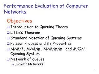
Outline • Introduction • Stochastic Modeling vs. Operational Analysis • Basic Performance Results • Utilization Law • Service Demand Law • The Forced Flow Law • Little's Law • Interactive Response Time Law • Bounds on Performance • Using QN Models • Concluding Remarks • Exercises • Bibliography
Introduction (1) • Chapter 2 introduced the basic framework that will be used throughout the book to think about performance issues in computer systems: • queuing networks. • That chapter concentrated on the • qualitative aspects of these models and • looked at how a computer system can be mapped into a network of queues. • This chapter focuses on the quantitative aspects of these models and
Introduction (2) • Introduce the input parameters and performance metrics that can be obtained from the QN models. The notions of • service times, • arrival rates, • service demands, • utilization, • response time, • queue lengths, • throughput, and • waiting time are discussed here in more precise terms.
Stochastic Modeling vs. Operational Analysis • SM • Ergodic stationary Markov process in equilibrium. • Coxian distributions of service times. • independence in service times and routing. • OA • finite time interval • measurable quantities • testable assumptions OA made analytic modeling accessible to capacity planners in large computing environments.
Application and Analysis of QN • Applications • System Sizing; Capacity Planning; Tuning • Analysis Techniques • Global Balance Solution • Massive sets of Simultaneous Linear Equations • Bounds Analysis • Asymptotic Bounds (ABA), Balanced System Bounds (BSB) • Solutions of “Separable” Models • Exact (Convolution, eMVA) • Approximate (aMVA) • Generalizations beyond “Separable” Models • aMVA with extended equations
Basic Performance Results (1) • This section presents the approach known as operational analysis [1], used to establish relationships among quantities based • on measured or • known data about computer systems. • To see how the operational approach might be applied, consider the following motivating problem.
Motivating Problem • Motivating problem:Suppose that during an observation period of 1 minute, • a single resource (e.g., the CPU) is observed to be busy for 36 sec. • A total of 1800 transactions are observed to arrive to the system. • The total number of observed completions is 1800 transactions (i.e., as many completions as arrivals occurred in the observation period). • What is the performance of the system (e.g., • the mean service time per transaction, • the utilization of the resource, • the system throughput)?
Measured Quantities Operational Variables • The following is a partial list of such measured quantities: • T: length of time in the observation period • K: number of resources in the system • Bi: total busy time of resourcei in the observation period T • Ai: total number of service requests (i.e., arrivals) to resource i in the observation period T • A0: total number of requests submitted to the system in the observation period T • Ci: total number of service completions from resource i in the observation period T • C0: total number of requests completed by the system in the observation period T
Derived Variables • From these known measurable quantities, called operational variables, a set of derived quantities can be obtained. A partial list includes the following: • Si: mean service time per completion at resource i; Si = Bi /Ci • Ui: utilization of resource i; Ui = Bi /T • Xi: throughput (i.e., completions per unit time) of resource i; Xi = Ci /T • i: arrival rate (i.e., arrivals per unit time) at resourcei; i= Ai /T • X0: system throughput; X0 = C0 /T • Vi: average number of visits (i.e., the visit count) per request to resource i; Vi = Ci /C0
Operational Analysis of motivating problem (1) • Using the notation above, the motivating problem can be formally stated and solved in a straightforward manner using operational analysis. • The measured quantities are:
Operational Analysis motivating problem (2) • Thus, the derived quantities are :
Multiple Class • The notation presented above can be easily extended to the multiple class case by considering that R is the number of classes and by adding the class number r (r = 1, ···, R) to the subscript. • For example, • Ui,r is the utilization of resource i due to requests of class r and • X0,r is the throughput of class r requests.
Operational Law • The subsections that follow discuss several useful relationships called: operational laws between operational variables. • Utilization Law, • Service Demand Law, • The Forced Flow Law, • Little's Law, • Interactive Response Time Law,
Utilization Law • As seen above, the utilization of a resource is defined as Ui = Bi /T • Dividing the numerator and denominator of this ratio by the number of completions from resource i, Ci, during the observation interval, yields (3.2.1 )
Utilization Law and Throughput • The ratio Bi/Ciis simply the average time that the resource was busy for each completion from resource i, i.e., the average service time Siper visit to the resource. • The ratio T/Ci is just the inverse of the resource throughput Xi. • Thus, the relation known as the Utilization Law can be written as: (3.2.2)
Utilization Law (3) • If the number of completions from resource i during the observation interval T is equal to the number of arrivals in that interval, i.e., if Ci = Ai, then Xi = i and the relationship given by the Utilization Law becomes Ui = Sixi. • If resource i has m servers, as in a multiprocessor, • the Utilization Law becomes Ui = (Six Xi)/m. • The multiclass version of the Utilization Law is Ui,r = Si,rx Xi,r .
Example 3.1. (1) • The bandwidth of a communication link is 56,000 bps and it is used to transmit 1500-byte packets that flow through the link at a rate of 3 packets/second. • What is the utilization of the link? • Start by identifying the operational variables provided or that can be obtained from the measured data. • The link is the resource (K = 1) for which the utilization is to be computed. • The throughputof that resource,X1, is 3 packets/second. • What is the average service time per packet?
Example 3.1. (2) • In other words, what is the average transmission time? • Each packet has 1,500 bytes/packet x 8 bits/byte = 12,000 bits/packet. • Thus, it takes 12,000 bits/56,000 bits/sec = 0.214 sec to transmit a packet over this link. • Therefore, S1 = 0.214 sec/packet. • Using the Utilization Law, we compute the utilization of the link as S1 x X1= 0.214 x 3 = 0.642 = 64.2%.
Example 3.2. (1) • Consider a computer system with one CPU and three disks used to support a database server. • Assume that all database transactions have similar resource demands and that the database server is under a constant load of transactions. • Thus, the system is modelled using a single-class closed QN, as indicated in Fig. 3.1. • The CPU is resource 1 and the disks are numbered from 2 to 4. • Measurements taken during one hour provide the number of transactions executed (13,680), • the number of reads and writes per second on each disk and their utilization, as indicated in Table 3.1.
Example 3.2. (2) • What is the average service time per request on each disk? • What is the database server's throughput? Figure 3.1. Closed QN model of a database server.
Example 3.2. (3) • The throughput of each disk, denoted by Xi (i = 2, 3, 4), is the total number of I/Os per second, i.e., the sum of the number of reads and writes per second. • This value is indicated in the fourth column of the table. • Using the Utilization Law, the average service time is computed as Si as Ui/Xi. • Thus, S2 = U2/X2 = 0.30/32 = 0.0094 sec, • S3 = U3/X3 = 0.41/36 = 0.0114 sec, and • S4 = U4/X4 = 0.54/50 = 0.0108 sec. • The throughput, X0, of the database server is given by X0 = C0/T = 13,680 transactions/3,600 seconds = 3.8 tps.
Service Demand Law (1) • The service demand, denoted as Di, is defined as the total average time spent by a typical request of a given type obtaining service from resource i. • Throughout its existence, a request may visit several devices, possibly multiple times. • However, for any given request, its service demand is the sum of all service times during all visits to a given resource. • Note that, by definition, service demand does not include queuing time since it is the sum of service times. • If different requests have very different service times, using a multiclass model is more appropriate.
Service Demand Law (2) • In this case, define Di,r, as the service demand of requests of class r at resource i. • To illustrate the concept of service demand, consider that six transactions perform three I/Os on a disk. • The service time, in msec, for each I/O and each transaction is given in Table 3.2. • The last line shows the sum of the service times over all I/Os for each transaction. • The average of these sums is 36.2 msec. • This is the service demand on this disk due to the workload generated by the six transactions.
Table 3.2. Service times in msec for six requests. Each transactions performs three I/Os on a disk. Service demand on this disk due to the workload generated by the six transactions. (33+41+36+32+36+39)/6=36.2 msec.
Service Demand Law (3) • By multiplying the utilization Ui of a resource by the measurement interval T one obtains the total time the resource was busy. • If this time is divided by the total number of completed requests, C0, the average amount of time that the resource was busy serving each request is derived. • This is precisely the service demand. So, • This relationship is called the Service Demand Law, which can also be written as Di = Vix Si . (3.2.3)
Service Demand Law (4) • By definition of the service demand (and since Di = Ui /X0 = (Bi /T)/(C0 /T) = Bi /C0 = (Cix Si )/C0 = (Ci /C0) x Si = Vix Si). • In many cases, Eq. (3.2.3) indicates that the service demand can be computed directly from the device utilization and system throughput. • The multiclass version of the Service Demand Law is Di,r = Ui,r /X0,r = Vi,rx Si,r.
Example 3.3. (1) • A Web server is monitored for 10 minutes and its CPU is observed to be busy 90% of the monitoring period. • The Web server log reveals that 30,000 requests are processed in that interval. • What is the CPU service demand of requests to the Web server? • The observation period T is 600 (= 10 x 60) seconds.
Example 3.3. (2) • The Web server throughput, X0, is equal to the number of completed requests C0 divided by the observation interval; • X0 = 30,000/600 = 50 requests/sec. • The CPU utilization is UCPU = 0.9. • Thus, the service demand at the CPU is • DCPU = UCPU/X0 = 0.9/50 = 0.018 seconds/request.
Example 3.4. • What are the service demands at the CPU and the three disks for the database server of Example 3.2 • assuming that the CPU utilization is 35% measured during the same one-hour interval? • Remember that the database server's throughput was computed to be 3.8 tps. • Using the Service Demand Law and the utilization values for the three disks shown in Table 3.1, yields: • DCPU = 0.35/3.8 = 0.092 sec/transaction, • Ddisk1 = 0.30/3.8 = 0.079 sec/transaction, • Ddisk2 = 0.41/3.8 = 0.108 sec/transaction, and • Ddisk3 = 0.54/3.8 = 0.142 sec/transaction.
The Forced Flow Law (1) • There is an easy way to relate the • throughput of resource i, Xi, • to the system throughput, X0. • Assume for the moment that every transaction that completes from the database server of Example 3.2 performs an average of two I/Os on disk 1. • That is, suppose that for every one visit that the transaction makes to the database server, it visits disk 1 an average of two times. • What is the throughput of that disk in I/Os per second?
The Forced Flow Law (2) • Since 3.8 transactions complete per second (i.e., the system throughput, X0) and each one performs two I/Os on average on disk 1, • the throughput of disk 1 is 7.6 (= 2.0 x 3.8) I/Os per second. • In other words, the throughput of a resource (Xi) is equal to the average number of visits (Vi) made by a request to that resource multiplied by the system throughput (X0). • This relation is called the Forced Flow Law: • The multiclass version of the Forced Flow Law is: Xi,r = Vi,rx X0,r. (3.2.4)
Example 3.5. • What is the average number of I/Os on each disk in Example 3.2? • The value of Vi for each disk i, according to the Forced Flow Law, can be obtained as Xi/X0. • The database server throughput is 3.8 tps and the throughput of each disk in I/Os per second is given in the fourth column of Table 3.1. • Thus, V1 = X1/X0 = 32/3.8 = 8.4 visits to disk 1 per database transaction. • Similarly, V2 = X2 /X0 = 36/3.8 = 9.5 and • V3 = X3/X0 = 50/3.8 = 13.2.
Little's Law (1) • Little's result states that the average number of folks in the pub (i.e., the queue length) is equal to the departure rate of customers from the pub times the average time each customer stays in the pub (see Fig. 3.2).
Little's Law (2) • This result applies across a wide range of assumptions. • For instance, consider a deterministic situation where a new customer walks into the pub every hour on the hour. • Upon entering the pub, suppose that there are three other customers in the pub. • Suppose that the bartender regularly kicks out the customer who has been there the longest, every hour at the half hour. • Thus, a new customer will enter at 9:00, 10:00, 11:00, ..., and • the oldest remaining customer will be booted out at 9:30, 10:30, 11:30, ....
Little's Law (3) • It is clear that the average number of persons in the pub will be , • since 4 customers will be in the pub for the first half hour of every hour and • only 3 customers will be in the pub for the second half hour of every hour. • The departure rate of customers at the pub is one customer per hour. • The time spent in the pub by any customer is hours. Thus, via Little's Law:
Little's Law (4) • Also, it does not matter which customer the bartender kicks out. • For instance, suppose that the bartender chooses a customer at random to kick out. • We leave it as an exercise to show that the average time spent in the pub in this case would also be hours. • [Hint: the average time a customer spends in the pub is one half hour with probability 0.25, one and a half hours with probability (0.75)(0.25) = 0.1875 (i.e., the customer avoided the bartender the first time around, but was chosen the second), two and a half hours with probability (0.75)(0.75)(0.25), and so on.]
Little's Law (5) • Little's Law applies to any "black box", which may contain an arbitrary set of components. • If the box contains a single resource (e.g., a single CPU, a single pub) or if the box contains a complex system (e.g., the Internet, a city full of pubs and shops), Little's Law holds. • Thus, Little's Law can be restated as (3.2.5 )
Little's Law (6) • For example, consider the single server queue of Fig. 3.3. • Let the designated box be the server only, excluding the queue. • Applying Little's Law, the average number of customers in the box is interpreted as the average number of customers in the server. • The server will either have a single customer who is utilizing the server, or the server will have no customer present. • The probability that a single customer is utilizing the server is equal to the server utilization. • The probability that no customer is present is equal to the probability that the server is idle.
Little's Law (7) • Thus, the average number of customers in the server equals: • This simply equals the server's utilization. • Therefore, the average number of customers in the server, N s, equals the server's utilization. • Thus, with this interpretation of Little's Law, • This result is simply the Utilization Law! • Now consider that the box includes both the waiting queue and the server. (3.2.6 )
Little's Law (8) • The average number of customers in the box (waiting queue + server), denoted by Ni, is equal, according to Little's Law, to the average time spent in the box, which is the response time Ri, times the throughput Xi. • Thus, Ni = Rix Xi. • Little's Law indicates that • ,where is the average number of customers in the queue and • Withe average waitingtime in the queue prior to receiving service.
Example 3.6. (1) • Consider the database server of Example 3.2 and assume that during the same measurement interval the average number of database transactions in execution was 16. • What was the response time of database transactions during that measurement interval? • The throughput of the database server was already determined as being 3.8 tps. • Apply Little's Law and consider the entire database server as the box.
Example 3.6. (2) • The average number in the box is the average number N of concurrent database transactions in execution (i.e., 16). • The average time in the box is the average response time R desired. • Thus, R = N/X0 = 16/3.8 = 4.2 sec.
Interactive Response Time Law (1) • Consider an interactive system composed of • M clients, • average think time is denoted by Z and • average response time is R. • See Fig. 3.4. • The think time is defined as the time elapsed since a customer receives a reply to a request until a subsequent request is submitted. • The response time is the time elapsed between successive think times by a client.
Interactive Response Time Law (2) • Let and be the average number of clients thinking and waiting for a response, respectively. • By viewing clients as moving between workstations and the database server, depending upon whether or not they are in the think state, and represent the average number of clients at the workstations and at the database server, respectively. • Clearly, since a client is either in the think state or waiting for a reply to a submitted request. • By applying Little's Law to the box containing just the workstations, • Since the average number of requests submitted per unit time (throughput of the set of clients) must equal the number of completed requests per unit time (system throughput X0). (3.2.7)