Download

1 / 64
640 likes | 900 Views
Longitudinal Data Analysis for Social Science Researchers Introduction to Panel Models. www.longitudinal.stir.ac.uk. SIMPLE TABLE – PANEL DATA. Women in their 20s in 1991 – Ten Years Later. BEWARE. BEWARE. Traditionally used in social mobility work

E N D
Longitudinal Data Analysis for Social Science ResearchersIntroduction to Panel Models www.longitudinal.stir.ac.uk
Women in their 20s in 1991 – Ten Years Later BEWARE BEWARE
Traditionally used in social mobility work • Can be made more exotic for example by incorporating techniques from loglinear modelling (there is a large body of methodological literature in this area)
Change Score • Less likely to use this approach in mainstream social science • Understanding this will help you understand the foundation of more complex panel models (especially this afternoon)
Vector of explanatory variables and estimates Yi 1 = b’Xi1 + ei1 Outcome 1 for individual i Independent identifiably distributed error
EQUATION FOR TIME POINT 2 Vector of explanatory variables and estimates Yi 1 = b’Xi1 + ei1 Outcome 1 for individual i Independent identifiably distributed error
Considered together conventional regression analysis in NOT appropriate Yi 1 = b’Xi1 + ei1 Yi 2 = b’Xi2 + ei2
Change in Score Yi 2 - Yi 1 = b’(Xi2-Xi1) + (ei2 - ei1) Here theb’is simply a regression on the difference or change in scores.
Change in Score Yi 2 - Yi 1 = b’(Xi2-Xi1) + (ei2 - ei1) Difference or change in scores (bfihhmn – afihhmn) Here theb’is simply a regression on the difference or change in scores.
Models for Multiple Repeated Measures “Increasingly, I tend to think of these approaches as falling under the general umbrella of generalised linear modelling (glm). This allows me to think about longitudinal data analysis simply as an extension of more familiar statistical models from the regression family. It also helps to facilitate the interpretation of results.”
Some Common Panel Models(STATA calls these Cross-sectional time series!) Binary Y Logit xtlogit (Probit xtprobit) Count Y Poisson xtpoisson (Neg bino xtnbreg) Continuous Y Regression xtreg
As social scientists we are often substantively interested in whether a specific event has occurred.Therefore for the next 30 minutes I will mostly be concentrating on models for binary outcomes
Recurrent events are merely outcomes that can take place on a number of occasions. A simple example is unemployment measured month by month. In any given month an individual can either be employed or unemployed. If we had data for a calendar year we would have twelve discrete outcome measures (i.e. one for each month).
Consider a binary outcome or two-state event 0 = Event has not occurred 1 = Event has occurred In the cross-sectional situation we are used to modelling this with logistic regression.
UNEMPLOYMENT AND RETURNING TO WORK STUDY – A study for six months 0 = Unemployed; 1 = Working
Months 1 2 3 4 5 6obs 1 0 0 0 0 0Employed in month 1 then unemployed
Months 1 2 3 4 5 6obs 0 0 0 0 0 1Unemployed but gets a job in month six
Here we have a binary outcome – so could we simply use logistic regression to model it?Yes and No – We need to think about this issue.
POOLED CROSS-SECTIONAL LOGIT MODEL x it is a vector of explanatory variables and b is a vector of parameter estimates
We could fit a pooled cross-sectional model to our recurrent events data.This approach can be regarded as a naïve solution to our data analysis problem.
Months Y1 Y2obs 0 0 Pickle’s tip - In repeated measures analysis we would require something like a ‘paired’ t test rather than an ‘independent’ t test because we can assume that Y1 and Y2 are related.
Repeated measures data violate an important assumption of conventional regression models. The responses of an individual at different points in time will not be independent of each other.
The observations are “clusters” in the individual SUBJECT Wave A Wave B Wave C Wave D Wave E REPEATED MEASURES / OBSERVATIONS
Repeated measures data violate an important assumption of conventional regression models. The responses of an individual at different points in time will not be independent of each other. This problem has been overcome by the inclusion of an additional, individual-specific error term.
POOLED CROSS-SECTIONAL LOGIT MODEL PANEL LOGIT MODEL (RANDOM EFFECTS MODEL) Simplified notation!!!
For a sequence of outcomes for the ith case, the basic random effects model has the integrated (or marginal likelihood) given by the equation.
The random effects model extends the pooled cross-sectional model to include a case-specific random error term this helps to account for residual heterogeneity.
Davies and Pickles (1985) have demonstrated that the failure to explicitly model the effects of residual heterogeneity may cause severe bias in parameter estimates. Using longitudinal data the effects of omitted explanatory variables can be overtly accounted for within the statistical model. This greatly improves the accuracy of the estimated effects of the explanatory variables.
An simple example – Davies, Elias & Penn (1992)The relationship between a husband’s unemployment and his wife’s participation in the labour force
Four waves of BHPS dataMarried Couples in their 20s (n=515; T=4; obs=2060) Summary information… 56% of women working (in paid employment) 59% of women with employed husbands work 23% of women with unemployed husbands work 65% of women without a child under 5 work 48% of women with a child under 5 work
First glimpse at STATA • Models for panel data • STATA – unhelpfully calls this ‘cross-sectional time-series’ • xt commands suite
STATA CODE Cross-Sectional Model logit y mune und5 Cross-Sectional Model logit y mune und5, cluster (pid)
xtdes, i(pid) t(year) xtdes, i(pid) t(year) pid: 10047093, 10092986, ..., 19116969 n = 515 year: 91, 92, ..., 94 T = 4 Delta(year) = 1; (94-91)+1 = 4 (pid*year uniquely identifies each observation) Distribution of T_i: min 5% 25% 50% 75% 95% max 4 4 4 4 4 4 4 Freq. Percent Cum. | Pattern ---------------------------+--------- 515 100.00 100.00 | 1111 ---------------------------+--------- 515 100.00 | XXXX
xtdes, i(pid) t(year) xtdes, i(pid) t(year) pid: 10047093, 10092986, ..., 19116969 n = 515 year: 91, 92, ..., 94 T = 4
xtdes, i(pid) t(year) Delta(year) = 1; (94-91)+1 = 4 (pid*year uniquely identifies each observation)
xtdes, i(pid) t(year) Distribution of T_i: min 5% 25% 50% 75% 95% max 4 4 4 4 4 4 4
xtdes, i(pid) t(year) Freq. Percent Cum. | Pattern ---------------------------+--------- 515 100.00 100.00 | 1111 ---------------------------+--------- 515 100.00 | XXXX Note: this is a balanced panel
xtdes, i(pid) t(year) xtdes, i(pid) t(year) pid: 10047093, 10092986, ..., 19116969 n = 515 year: 91, 92, ..., 94 T = 4 Delta(year) = 1; (94-91)+1 = 4 (pid*year uniquely identifies each observation) Distribution of T_i: min 5% 25% 50% 75% 95% max 4 4 4 4 4 4 4 Freq. Percent Cum. | Pattern ---------------------------+--------- 515 100.00 100.00 | 1111 ---------------------------+--------- 515 100.00 | XXXX