
Power
Power. We all know what P(Type I Error) = is: = P (rej. H 0 / H 0 true) = P(Type II Error) = P (acc. H 0 / H 0 false). Power is : “the ability to detect out a small deviation from the hypothesized value.” “The test which can detect a smaller deviation is the more powerful one.”

Power
E N D
Presentation Transcript
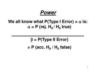
Power We all know what P(Type I Error) = is: = P (rej. H0 / H0 true) = P(Type II Error) = P (acc. H0 / H0 false)
Power is : “the ability to detect out a small deviation from the hypothesized value.” “The test which can detect a smaller deviation is the more powerful one.” What is “power” in terms of , b ?
H0 true H0 false Type II error No Error 1- we accept H0 Type I error No Error 1- we reject H0 = P (acc. H0 / H0 false) 1- = P (rej. H0 / H0 false) = a correct conclusion 1- = “POWER” (of a test)
1 R (• j - ••)2 C For ANOVA (with one factor) we have, POWER = f ( , 1, 2, = significance level 1 = df of numerator (of Fcalc) 2 = df of denominator (of Fcalc) “Non-Centrality Parameter” = A MEASURE OF HOW DIFFERENT THE ’s ARE FROM ONE ANOTHER (includes “sample size” by including R & C)
1 - = Function of a distribution called “non-central F dist’n” (which is NOT the same as the regular F distribution) However, typically, we don’t know or the values. So — in practice, you need to “estimate” from data and “suppose” a value of for purposes of finding POWER
10(52 + 02+ 52) 3 500 3 12.9 5 Example: One factor ANOVA with = .05, R = 10, C = 3. We decide that a working estimate of = 5 and that we (arbitrarily) choose to calculate (1-) assuming that the ’s are each 1• apart. (eg., 17 22 27). Then, 1/2 ( 1 5 ) = 1/2 ( ) 1 5 = 2.58 = =
We have = 2.58 1 = 2 (3 col) 2 = 27 (30-3) = .05 Now go to “Power Tables”: eg., the one for 1 = 2 (they are “indexed” by the value of 1): This table is for = .05 and for = .01, and for various values of 2 and.
POWER ( 2) at 1 = 2 See next page for chart ) ( 2 = 30, = 2.6 POWER .976 = .05, Our Answer:
Accept H0 = All column means are the same. All column means are each “<5” apart with “97.6%” confidence.
FINDING “REQUIRED”SAMPLE SIZE Given C, , 1-, and “” we can find the minimum sample size required, in terms of R, the number per column. = Max (•j) – min (•j) = Range of ’s
Sometimes one estimates and separately; sometimes one estimates the ratio and not necessarily the separate values. A common choice of is 2 (i.e., the range of ’s is 2 standard deviations). C = 3 = .05 = .90 = 2 Example: R = 8
(1-a) Confidence Interval (C.I.) • For • j: • For • j- • k:
If s is unknown, • Replace s by • Replace Z1-a/2 by t1-a/2 where the df of t is the df of Error.