Download
1 / 31
310 likes | 336 Views
Delve into the intricate world of black holes and gravitational waves using cutting-edge numerical relativity simulation techniques. Learn the fundamentals of gravity, the formation and behavior of black holes, and the detection of gravitational waves using advanced tools. Discover how numerical relativity aids in predicting gravitational waveforms, simulating astrophysical phenomena, and uncovering new aspects of general relativity. Explore the tools and methodologies essential for visualizing complex data and understanding the curvature of space-time. Engage in a journey of scientific exploration and innovation, shedding light on the mysteries of the universe.

E N D
Maria Babiuc-Hamilton Department of Physics BLACK HOLES SIMULATION and visualization Marshall University, Huntington, WV – April 7, 2011
The Elusiveness Of Gravity • What is Gravity? Not an attraction force! • Matter distorts the space-time geometry • This distorted geometry makes matter move
Matter Is Geometry • Einstein summarizes his Theory of General Relativity • “People before me believed that if all the matter in the universe were removed, only space and time would exist. My theory proves that space and time would disappear along with matter” • Empty space-time is flat Arrangement of matter and energy Curvature of space-time (geometry)
What Are Black Holes • First and foremost implication of Einstein’s Theory of General Relativity • Space-time is so distorted by mass, that nothing, not even light can escape! • The radius of no return forms the event horizon. • The center is a “tear” in the fabric of space-time
Where Are Black Holes • Formed from the supernova explosion of massive stars. • “Supermassive” black holes at the center of all galaxies. • Black holes can be: • stationary or spinning , • isolated or in an orbiting pair.
Gravitational Waves • Vibration in space-time due to accelerated mass, like: • Supernovae explosions, • Black holes spinning or in pairs • Why study it? • New insights into: • the formation of galaxies • behavior, structure and history of space-time • test and validate alternative theories of gravity
A New Astronomy Laser Interferometer Space Array -not yet launched- • Normal Astronomy sees with “light waves” (visible, radio, x-rays…) • Gravitational Wave Astronomy “sees” with gravitational waves • What will we “see”? • colliding black holes, • supernova explosions, • the birth of the universe • the structure of space-time Laser Interferometer Gravitational-wave Observatory (LIGO)
What Is Detected • LIGO and LISA will detect any small vibration, not only gravitational waves! • Need models to know what to look for and tell the signal from the noise. • Templates are essential for detection
Numerical Relativity • Uses computer codes to simulate black hole collisions and predict the gravitational wave signal for gravitational wave observatories • Key tool to: • Predict gravitational waveforms • Simulate known astrophysical phenomena • Discover new phenomena in general relativity
Simulation Tools • Cactus Code: • Programming environment for High Performance Computing • Enables parallel computation on supercomputers • Allows modular code development and large scientific collaborations • Einstein Toolkit: • Modular computer codes for Astrophysics • Solves Einstein Equations and simulates space-time • Built-in codes that allow flexible input and output
Visualization Tools • The simulation is run and a lot of numbers are produced: the DATA. • A picture is worth a thousand “numbers.” • We use the following free visualization tools to look at the data: GRACE: 2D plotting tool for X windows, running in all systems. http://plasma-gate.weizmann.ac.il/Grace/ GNUPLOT: command line interactive plotting function, 1/2/3 D http://gnuplot.en.softonic.com/ VISIT: visualization tool for parallel, interactive visualization of data https://wci.llnl.gov/codes/visit/
Einstein Equations Geometry (space-time Curvature) Matter (mass and energy) Gmn= 8pTmn • Black holes are simple pure vacuum! Gmn= Rmn – 1/2gmnR = 0 • There is no known stable algorithm Metric Tensor Curvature Scalar Einstein Tensor Curvature Tensor
Inherent Difficulty • How to simulate the singularity in a stable way • Coordinates need to be constructed during evolution • Conservation laws impose constraints and overdetermine the evolutions
Ingredients of Simulation • Decompose the space-time in space+time (foliate) • Evolution: • Solve constraints initially • Evolve data • Reconstruct the space-time • Extract the physics. Obtain Einstein Equations on the next slice Evolve (step-up) In time Give Einstein Equations on the Initial Slice =foliate=
Initial Data • General relativity depends on initial conditions • Initial data is specified on a slice of space-time that sufficiently determine the future evolution. Brill-Lindquist Schwarzchild Boyer-York Wormhole
Harmonic Evolution • The coordinates xmsatisfy a wave equation xm=0 • The vacuum Einstein equations reduce to 10 wave equations acting on the metric components gmn D’Alembertian
Numerical Approximations • Problem:how to model infinite continuum space-time partial derivative with finite discrete numerical representation? • fromCalculustoAlgebra du/dx = u(x+h)-u(x-x)/2h +O(h2) • The accuracy of the simulation is given by the convergence of the code to the analytical solution.
Well Posedness • Given a system of partially differential equations, well posedness means that: • A solution exists • The solution is unique • Plus, the solution should be stable = depend continuously on the initial data.
Well Posedness • Problems even with a “well posed” formulation: • Grid induces high frequency modes • Constraint violation exponential modes • Solutions: • Dissipation to control the high frequency modes • Constraint adjustments to control exponential modes
Marching To Infinity • How to approach infinity when given only a finite amount of computer power and time? • Go on a SUPECOMPUTER! • One has to stop somewhere! • Truncate the computational domain by introducing an artificial outer boundary sufficiently far from both the region where data is extracted.
When Is It Far Enough? • The artificially introduced outer boundary is too far enough if: • is causally disconnected from the dynamical parts of the simulation • accurately extrapolate the gravitational waveform at infinity • accounts for errors and perturbations without interfering with the simulated physics
The Boundary Problem • Must solve again the “well-posedness” problem. • The outer boundary must be well posed: • a unique solution, continuously dependent on the initial data,must exist • Moreover, the boundary must • Control incoming radiation • Be compatible with the constraints Artificial boundary due to limited resources Boundary data needs to be Well-posed
Exploring Solutions • Developed techniques to suppress exponentially growing instabilities • Implemented stable and convergent outer boundary conditions of absorbing type • Introduced a new formulation of constraint preserving boundary conditions for the general case of “moving boundaries” • Implemented and testes with a 3D finite-difference general harmonic code • Building a pilot computational code with the purpose of introducing electromagnetic field and matter
Show Me The Physics! • We proved the simulation is reliable • The data extracted will give information on the: • motion of the Black Hole • properties of the Black Hole Horizon • Problem: The emitted gravitational wave radiation has to be extracted at infinity, or adequately far from coalescing binary black hole!
A Rotating Black Hole The lapse for the whole run The metric over the whole run
Two Inspiral Black Holes The curvature The lapse for the whole run
The Characteristic Approach • Choose a slicing condition to include a “null infinity” in the computational domain. • Null infinity =the set of points which are approached asymptotically by light rays • The radial coordinate is “compactified”: r->x = r/(r+R) • The waveform is evolved along the light ray and computed at null infinity
Binary-Black Hole Waveforms • Waveform extraction form the inspiral and merger of two non-spinning black holes of equal mass The gravitational wave at the peak of the signal The principal mode of the wave in time