Download
1 / 36
360 likes | 517 Views
Class 2. Review major points from class 1 New Material Reaction (receptor binding) kinetics Diffusion Einstein relation Fick’s Law SPR sensors. Review of last week B iological molecules are often complex polymers e.g. proteins, DNA

E N D
Class 2. Review major points from class 1 New Material Reaction (receptor binding) kinetics Diffusion Einstein relation Fick’s Law SPR sensors
Review of last week Biological molecules are often complex polymers e.g. proteins, DNA Interact via fundamental forces (e.g. electrostatics) but these are often shielded by ions in solution -> complex weak interactions ~kBT over short distances (e.g hydrogen bonds, hydrophobic effects, base pairing) Lots of molecule-specific interactions Boltzman distribution – chance that molecule is in state with energy E ~ exp(-E/kBT)
Did not review derivation of Boltzman distribution But could for those with mathematical bent… (if time and interest at end of class) New topic – binding kinetics
Consider a microtiter well sensor coated with antibodies filled with sample containing ligand molecules “free” ligand molecule L Volume of liquid sample = V “free” antibody molecule Ab antibody that has bound ligand AbL
Ab + L <-> AbL Let [AbT] = total # antibody molecules on sensor surface/ sensor vol V (in some sense the Ab concentration) [LT] = total # of ligand molecules in the sensor/V note [ ] indicates concentration [Ab(t)] = concentration of antibody molecules that have not bound ligand at time t, i.e. that are free to bind L [L(t)] = concentration of ligand molecules that have not bound antibody at time t, i.e. that are free to bind Ab
By conservation of molecules [AbT] = [Ab] + [AbL] (1) [LT] = [L] + [AbL] (2) Simple model for Ab + L AbL d/dt [AbL] = kon [Ab] [L] – koff [AbL] at equilibrium, d/dt [AbL] = 0 => kon [Ab] [L] = koff [AbL] [Ab] [L]/[AbL] = koff/kon= KD (3) kon koff -> <-
Note (1), (2) and (3) are 3 eqns w/ 6 “variables”: ([AbT], [LT], [Ab], [L], [AbL], KD Frequently only interested in fraction of Abs that have bound L, i.e. [AbL]/[AbT] (or fraction of L that have bound Ab, i.e. [AbL]/[LT]) Then (1-3) can be rewritten (you should check this!): [AbL]/[AbT] = [L]/KD / (1 + [L]/KD) (4) [AbL]/[LT] = [Ab]/KD / (1 + [Ab]/KD) (5)
The “signal” from L binding (e.g. dye color in some ELISAs) is often proportional to the amount of ligand that binds, i.e. [AbL] or the rhs of 4 or 5 Then if you plot signal vs free Ab or L concentration, you get sigmoid curve, half max at [L] = KD (or [Ab]=KD) This can be used to determine the KD ½ max + ½ max + 1 1 signal signal [Ab]/KD [L]/KD
Units d/dt [AbL] = kon [Ab] [L] – koff [AbL] conversion factor CF chemistry SI units (SI = chem x CF) [X] M = moles/liter #/m3 6*1026 koff s-1 s-1 1 kon M-1s-1 = l/mole-s (#/m3)-1s-1 (6*1026)-1 KD Mm3/# KD is a measure of the strength of an interaction; the lower the KD, the tighter the binding; [X]/KD is unit-less kon is # reactive collisions/sec each molecule of Ab or L makes when it’s partner is at “unit” concentration signal [L]/KD
[AbL]/[AbT] = [L]/KD / (1 + [L]/KD) (4) [AbL]/[LT] = [Ab]/KD / (1 + [Ab]/KD) (5) Note when [L] << KD, fraction of Ab “bound” -> [L]/KD when [L]>> KD, fraction of Ab “bound” -> 1 High conc. of either free species, [L] or [Ab], “drives” its partner into a complex Eqns (1) – (3) are symmetric in Ab and L, so symmetry of 4 and 5 is expected
Caveat: (4) or (5) are useful when AbT (or LT) is in excess so that complex formation does not deplete the species in excess, i.e. [Ab] @ [AbT]) (or [L] @ [LT]) because you often know [AbT] or [LT] but not [Ab] or [L] [AbL]/[AbT] = [L]/KD / (1 + [L]/KD) (4) [AbL]/[LT] = [Ab]/KD / (1 + [Ab]/KD) (5) Example: If you want to measure ligand at pM conc. by ELISA, is (4) or (5) relevant? Assume KD is nM, you can pack antibodies on the plastic surface at 1012/cm2 (do you want high or low [AbT]?), a well has an area of ~0.1cm2, and sample volume is 100ml
If ligand is likely to be at nMconc, is (4) or (5) useful to measure KD? You don’t need to know [Ab] or [L] if you don’t care about KD and just want [LT] for an unknown by comparing the signal it gives to that from known concentrations [LT] of a standard Note [Ab] and [L] are not really symmetric because Ab is fixed and L is free to diffuse; the above treats the Ab as if it were free in solution at conc = # surface molecules/ vol; dicey!
If neither Ab nor L is in excess, it’s better to use (1) and (2) to eliminate [Ab] and [L] from (3), giving a quadratic eqn for [AbL]: [AbL]2 – [AbL] (KD + [LT] + [AbT]) + [AbT][LT] = 0 => [AbL] = -b/2 + (b2/4-c)1/2 Is the + or – solution non-physical? Hint: if [LT] = 0, what is c, and what must [AbL] be? You could use this to get [LT] if you measure signal (~{AbL]) and know KD and [AbT] c b
What is sensitivity (lowest detectable conc) in a good ELISA? How many molecules in 100ml sample @ 0.5pg/ml If MW = 2*104g/mole? If KD=nM and 1011 capture Abs/well, what fraction of ligand is bound? Hint: is Ab or L in excess? How does [Ab] cf to KD? * Sensitivity usually limited by noise from non-specific sticking of enzyme -> color
The simple model also gives kinetic information: d [AbL(t)]/dt = kon[AbT-AbL(t)] [LT – AbL(t)] – koff [AbL(t)] Suppose LT >> Ab so that LT – AbL(t) @ LT. Divide all terms by [AbT] Let f(t) = fraction of Ab bound at time t, f(t) = AbL(t)/AbT This gives simple diff eqn for f(t): f’(t) = -f(t) {(LTkon + koff)} + konLT
f’(t) = -f(t) {(LTkon + koff)} + konLT f(t) has simple solution: f(t) = A(1-e-Bt) where A = [LT/KD /(1 + LT/KD)] and B = konLT + koff (if you are unfamiliar with this, check by substitution) Plot of f(t) vs t A = LT /KD /(1 + LT/KD) fraction of Ab that bind L = f(t) time • = 1/B = koff-1/(1+LT/KD) Note f(t) exponentially approaches equil. value with characteristic time t
LT/KD /(1 + LT/KD) f(t) If LT << KD, t -> 1/koff If LT >> KD, t -> koff-1 KD/LT = 1/(konLT) typical values kon~ 104 - 106/Ms( =10-23 – 10-21 m3/s) koff~ 1/s to 10-3s KD~mM (weak) to nM (tight binding) If LT is not in excess, the diff. eqn. is not simple and requires numerical solution time t = koff-1/(1 + LT /KD)
What determines kon? Need digression to discuss Brownian motion and diffusion
Diffusion and Brownian motion • Why do molecules diffuse? • How far away do they go (on average) in time t? • Let <x2(t)> = av. displacement2 of molecule after time t • Why talk in terms of <x2(t)> instead of <x(t)>? • <x2(t)> =~ t Why not ~t2? They keep changing directions. • In 1-d, suppose molecule moves randomly +d every t sec • <(xnt)2> = <(x(n-1)t +d)2> = <(x(n-1)t)2 + 2x(n-1)td+ d2> = nd2 • since n = t/t, <x2(t)> = (d2/t)t =2Dtwhere D is diff. const. • Note D=d2/2thas units of m2/s. Time to diffuse x = x2/2D • How can we estimate D?
Deep connection between D and viscous drag: both are due to bombardment by adj. molecules Why do objects pushed at constant F move with constant velocity in viscous media rather than accelerate according to F = ma? Einstein suggested they do accelerate with a=F/m for short times, but then are struck sufficiently hard by other molecules that their velocity is randomized Let average time between velocity-randomizing collisions = t Terminal velocity (before next collision) = (F/m) t
Does this microscopic terminal velocity=macroscopic vdrift of body subject to force F in medium with viscosity h? In laminar flow, drag force on sphere radius r Fdrag = gv v = Fdrag/g where g = 6phr Stokes law h=viscosity, 10-3 Ns/m2 in water (viscosity = shear force/velocity gradient ^ to shear) If the two are the same, F/6phr=(F/m)t => t/m = 1/6phr Finally, all objects in thermal equilibrium have average kinetic energy mvx2 = kBT => vx= d/t = (kBT/m)1/2
This gives 3 relations between “microscopic” quantities d, t, m and “macroscopic” quantititesg (= 6phr), kBT, and D: d2/2t =D (4) t/m = 1/6phr (5) d/t = (kBT/m)1/2 (6) Use (4) and (5) to eliminate d and m in (6) -> D = kBT/6phr Einstein relation (lost factor of 2) This gives you D for a molecule in medium with viscosity h, if you can estimate its radius r (!)
Example: What is the diffusion constant in water for an antibody molecule whose radius is 3nm? viscosity of water h = 10-3 Ns/m2 (check units = F/area/gradient of velocity) kBT = 4*10-21J at room temperature (T~300oK) (useful to remember this for this course!) D = kBT/6phr = 4*10-21 J/(6*3.14*10-3*3*10-9Js/m2) = 6*10-11m2/s Note units! 100x larger virus has 100x smaller D since D~1/r
About how long does it take a 2nm molecule to diffuse 3mm? (approx. distance to surface in microtiter plate well)? t = x2/6D in 3dimensions = 9x10⁻⁶/6x10-10 = 104s (hours!) twice dimension # that’s why ELISA takes so long! Diffusion explains bulk flow of molecules down a concentration gradient c(x) | c(x+d) total flux ½ c(x) A d/t -> <- ½ c(x+d) A d/t net flux j D (# molecules crossing unit area per s) = {(c(x) – c(x+d))/d} (d2/2t) = -D dc/dx check that units agree! This is Fick’s Law
How does this relate to kon? Diffusion limited molecular collision rate is tricky to derive but consider that molecule of radius r diffusing distance r in time t = r2/6D collides with all ligand molecules in volume ~pr3 # collisions/s @ pr3[L]/(r2/6D) = 6D pr[L] = 6prkBT[L]/6phr @kBT[L]/h = kon [L] => kon = kBT/h = 4*10-21/10-3m3/s @ 2*109M-1s-1 Observed kon’s are ~ 104 – 106 M-1s-1, suggesting that only 1 in 103-105 collisions results in binding
How are kon’s measured? SPR (surface plasmon resonance) sensors is 1 way Quantitative details of SPR not important for this course, but try to get qualitative understanding
Surface plasmon resonance (SPR) sensors Like real-time immune capture assay Transduction method Sensing principle – light incident on glass surface > critical angle is totally reflected; if glass has thin metallic coating, evanescent wave in metal polarized in plane of incidence canexcite coherent movement of electrons on metal surface when resonance condition kx = ksp is met
Surface Plasmon Resonance – prism configuration 2 q Since kx = (w/c) n sin q = ksp, surface plasmon excited at particular incidence angle qr -> decrease in reflection intensity ksp very sensitive to n2~ mass bound to metal surface To first order, Dqr ~ Dm
How sensitive is Dqrto Dm? Typical sensitivity limit is ~1pg (~107 molecules for MW 105) in sensor area 1mm2 (roughly comparable to ELISA); this is equiv. to covering ~ 1/1000th of surface Less sensitive per bound molecule when ligand is small (signal ~mass bound) but still can be used to study protein-drug interactions Advantages cf to ELISA real time results, don’t need label, more automatable get kinetic parameters kon, koff, KD, and LT as well as L Disadvantages – cost ~$100K/machine, expensive flow cells
Lots of info available on web and from vendors, e.g. Biacore, now part of GE http://www.biacore.com/lifesciences/technology/introduction/following_interaction/index.html http://www.biacore.com/lifesciences/technology/introduction/data_interaction/index.html Note SPR facilitates depositing your own receptors http://www.protein.iastate.edu/seminar/BIACore/ TechnologyNotes/TechnologyNote1.pdf http://www.bama.ua.edu/~chem/seminars/ student_seminars/fall08/f08-papers/ bokatzian-johnson-sem.pdf http://www.biosensingusa.com/Application101.html
Characteristic SPR binding curve data Conc that -> half max binding = KD Flow in analyte Flow in buffer (analyte elutes) charact. off time = 1/koff 1RU=10-4 degrees analyte conc. nM Can you estimate 1/koff from these curves? Can you estimate conc. that gives half max binding? Do they wait long enough to reach binding equilibrium?
Example – kinetic constants extracted from SPR data for binding of various engineered, antibody-like molecules to their targets Note ~106/Ms ~1/1000s ~nM
Note SPR provides “real-time” binding assay, so close to a reporter of events modeled in binding kinetics theory More complex phenomena revealed by SPR sensors E.g. as molecules adsorb to surface, they are depleted from region just above surface. What does this do to concentration near surface? To binding rate? # molecules that bind/s = konLs [Ab(t)] Does incoming flow keep Ls = LT? koffmay be underestimated because of rapid rebinding Need more detailed model of mass transport to extract KD, kon from raw data = topic in 2 weeks
SPR is work-horse for analysis of protein interactions in biochemistry labs/ pharmaceutical industry Does it need to be so expensive? Texas Instruments’ SPR chip - SPREETA Sensors and Actuators B 91 (2003) 266–274 Could you put one in cell phone?
References/reading Random Walks in Biology, Howard Berg, 1993 a great paperback, p. 5-11, 17-42 Chapter on diffusion in Nelson http://www.fas.harvard.edu/~scphys/nsta/viscosity_brownian.pdf Short chapter from Harvard class on Einstein relation
Next week Do homework problems on binding kinetics, diffusion Read general article on single-molecule ELISA to get basic idea, then article on theory of single-mol assay (in J of Immunol) for review of binding kinetics and state –of-the-art application See questions on theory article (on Blackboard) to help you digest it picka figure from this paper to discuss in class