Download
1 / 34
350 likes | 479 Views
Yield Revenue Management and Costly Consumer Search MOSCOW 2012 June 8. Simon P. Anderson, University of Virginia, USA a nd Yves Schneider, University of Lucerne Switzerland. Back-drop. Cruise-ship mergers; can they be pro-competitive? (D Scheffman ) Likewise, airlines, hotels, etc

E N D
Yield Revenue Management and Costly Consumer SearchMOSCOW 2012 June 8 Simon P. Anderson, University of Virginia, USA and Yves Schneider, University of Lucerne Switzerland
Back-drop • Cruise-ship mergers; can they be pro-competitive? (D Scheffman) • Likewise, airlines, hotels, etc • Yield Revenue Management: lots of OR, almost all monopoly • Competition is tough to analyze (Dudey, Varmas & Vettas)
Order of events • Monopoly problem • Duopoly, no search costs • Duopoly with search costs • non-binding then binding • Results with capacity choice • Some evidence • Discussion of assumptions
Take-aways • Duopoly can be worse than monopoly • Higher prices for duopoly • In presence of search costs
Monopoly problem • Simple version • L consumers arrive sequentially in given order, do not return • Valuations i.i.d. • Capacity K; ignore discounting • What do prices look like? • Rise / fall over time depending on previous success
Value V(Ɩ;k) • V(0;k) = 0 • V(Ɩ;k) = π Ɩ for k ≥ Ɩ (monopoly price & profit for each “period”) • V(Ɩ;1) : drop price over time until sell • V(Ɩ;k) concave in Ɩ and k (decreasing marginal benefits)
Solving value • Let valuations be drawn from F(p) in [0,1] with (1-F) being (-1)-concave Then program with Ɩ left is: V(Ɩ;k) = maxp { F(p)V(Ɩ-1;k) + (1-F(p))(p + V(Ɩ-1;k-1) } Two events. • Foc: p - (1-F(p))/f(p) = V(Ɩ-1;k) - V(Ɩ-1;k-1) • MR = MC governs choice over time • For linear demand, p = (1+MC)/2
Working backwards • Think of Ɩ falling and k falling as sales are made; work back from final states • Build up solution recursively
Linear demand, 3 consumers, k=2 • (k≥3 is just p=1/2 throughout), similarly • V(2;2)= ½ ; V(1;1)= V(1;2)=¼ (& V(0;k)=0) • ¿V(2;1) ? : MC of selling is V(1;1)-V(1;0)=¼ So price is 5/8. Hence the value V(2;1) is (5/8) V(1;1) + (3/8)(5/8 + V(1;0)) = 25/64 • To find p3,2, note MC is V(2;2)- V(2;1) = 7/64 • So price is 71/128 (etc!)
Price patterns: rises if a sale and falls if there was no sale
Duopoly analysis • Suppose capacities K1 and K2. • Consumers arrive sequentially, see both prices, buy from cheaper. Then disappear, never to return. • If one stocks out, the other firm is a monopoly henceforth (we already know the monopoly)
Duopoly, no search cost • If both capacities exceed Ɩ, prices are zero by standard Bertrand argument. • If one has stocked out, the other follows the monopoly program • The one with higher capacity may let the other win in order to precipitate getting the monopoly position
Duopoly example • Assume L=3, K1 = K2 = 2 • To solve this, we must find V1(2; k1, k2) and V2(2; k1, k2) • If no sale to Ɩ=3, values are zero henceforth • So consider V1(2; 2, 1) and V2(2; 2, 1) • If 1 makes the sale to Ɩ=2, both expect nothing thereafter, so 1 would rather 2 sells (“CTD”) • If 2 sells, then 1 is a monopoly after, with expected profit 1/4
Duopoly with no search cost, ctd • Hence 1’s opportunity cost is ¼, so 1 undercuts 2 at any higher price for Ɩ=2 • Equilibrium thus has p2 = ¼ and 1 Clears the Decks of 2 • Now consider Ɩ=3 • If neither sells, they both get nothing, if either sells, they BOTH get ¼.¾ continuation, plus whatever current revenue. • So they bid p3 down to zero (and not below)
Duopoly take-aways • “Clear-The-Decks”: exacerbate asymmetries, let other go first • Cournot-like capacity game • Lower prices than monopoly, higher welfare • More extended: not clear CTD holds; Vettas, Dudey unfinished (?) work
Duopoly with search costs • Suppose the first search / observation is free (and random across the 2 firms) • Second search costs c • Consumers know their order of arrival (e.g., time of day) and how much capacity is left at each firm • 2 cases; search cost prohibitive, or maybe binding • [recall Diamond Paradox]
Duopoly with positive search cost (c large) • Firm 1 is to max by choice of p1 ½{F(p₁)V₁(Ɩ-1;k₁,k₂)+(1-F(p₁))[p₁+V₁(Ɩ-1;k₁-1,k₂)]} + ½{F(p₂)V₁(Ɩ-1;k₁,k₂)+(1-F(p₂))V₁(Ɩ-1;k₁,k₂-1)} Note that 1 can’t affect second part, so just chooses price against first part; like the monopoly problem in structure (other’s impact through k₂) Solve by working back
(prohibitive) search cost example • Suppose Ɩ=3 & K1=K₂=1 • Last consumer, either a monopoly with profit ¼ or a duopoly with profit 1/8 (Diamond Para) and monopoly prices • Ɩ=2 : if no prior sale, what is opp. cost? 1/8 So price is 9/16 (above monopoly levels for 2 units of capacity and 2 consumers) • Similar for both firms, so now find p3
First find V₁(2;1,1) : • Recall V₁(Ɩ;k₁,k₂)= ½{F(p₁)V₁(Ɩ-1;k₁,k₂) +(1-F(p₁))[p₁+V₁(Ɩ-1;k₁-1,k₂)]} + ½{F(p₂)V₁(Ɩ-1;k₁,k₂) +(1-F(p₂))V₁(Ɩ-1;k₁,k₂-1)} • With now p1=p₂=9/16; so V₁(2;1,1)= ½{(9/16)(1/8)+(7/16)(9/16)} + ½{(9/16)(1/8)+(7/16)(1/4)} = 127 / 512
Firm 1 is to max by choice of p1 ½{F(p₁)V₁(2;1,1)+(1-F(p₁))[p₁+V₁(2;0,k₂)]} + ½{F(p₂)V₁(2;1,1)+(1-F(p₂))V₁(2;1,1)} And V₁(2;1,1) = 127/512 and V₁(2;0,k₂)=0; so opp. cost is 127/512 and price is 639/512 ≈ 0.624 (using monopoly pricing rule)
Example summarized • higher price under duopoly than monopoly (0.624 compared to 0.555) • duopolists also demand a higher p2 if no sale was made to first consumer (0.5625 compared to 0.5) • Joint expected profits of the duopolists are V₁(3;1,1)+V₂(3;1,1)≈0.691 monopolist has Vm(3;2)≈0.698
(more simply – higher duop OC) • 2 periods and one unit each • Monopoly would be price ½ each pd • Duopoly set higher prices first period because consumer won’t search, and also Opp. Cost is 1/8 profit at end • So price 9/16
Asymmetric capacities e.g. • Last e.g. had same prices, so no role for search • Suppose 2 consumers, K1=2, K₂=1. Find price path • If 2 sells out, 1 is then a monopolist for the last consumer remaining. Sets p1 = ½, profit ¼ • If 1 sells, Diamond result: p1 = ½, profit 1/8 each, same as if 1 doesn’t sell • So for Firm 1, p2 = ½ • Firm 2, opp cost is 1/8, so its p2 = 9/16 • Smaller firm has higher price (expected?) And its price is unconstrained if c≥ 1/16. Otherwise…
Asymmetric capacity; c < 1/16 • Then Firm 2 is constrained: candidate equil sets ½+c • Does Firm 1 want to deviate to CTD by setting a high price? NO • Never find CTD here, always want to be in contention, perhaps at high price
lower search costs discipline Lo-capacity firm, Lo is worse off, Hi better because Lo Clears quicker
Proposition 3. Let the duopolists be endowed with initial capacities K1 and K2, respectively. • If K1 + K2 ≥ L then a monopolist initially endowed with capacity K1 + K2 charges pm for each unit while duopolists always charge a price of pm or above. • Welfare is higher under monopoly than under duopoly.
K1 + K2 < L: numerical methods. Proposition 3 holds more generally: Result 1. Simulations for uniform valuations and search costs c = 0.05 confirm Proposition 3 for L < 100 and all capacity levels. (no reason to expect different results for L > 100, for different search costs, or for different distributions of valuations)
welfare • Lower for duopoly because higher prices • Reason is higher duopoly Opp. Cost • Still have a shot of a sale next time even if other still has capacity, because consumer may come to you first • Hence monopoly can be more efficient market form here
On (heroic) assumptions • Costless first search: standard in (early) search literature, otherwise Diamond hold-up - Stiglitz twist of down-slope demand: more complex here! (AR heterogeneous consumers?) • Consumer knows state: may know time of day of visit, but how know how much cap left? Diamond Paradox may “help” – don’t expect lower prices elsewhere, so don’t search
Sum-up • Competition can raise prices and lower welfare • Because higher opp. costs – firm can still sell later when monopoly has zero benefit from capacity • Context of capacity constraints and costly consumer search • Revenue management and oligopoly with (and without!) frictions deserves more work • www; role of comparison sites?