Download
1 / 38
410 likes | 736 Views
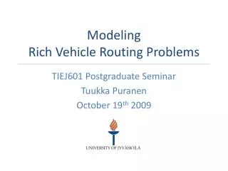
Modeling Rich Vehicle Routing Problems. TIEJ601 Postgraduate Seminar Tuukka Puranen October 19 th 2009. Contents. A tour on combinatorial optimization problems relevant to logistics design Vehicle Routing Problem and its variants The proposed model for VRP Analysis

E N D
Modeling Rich Vehicle Routing Problems TIEJ601 Postgraduate Seminar Tuukka Puranen October 19th 2009
Contents • A tour on combinatorial optimization problems relevant to logistics design • Vehicle Routing Problem and its variants • The proposed model for VRP • Analysis • Effects and possibilities of the new model • I will not talk about implementation, system design, optimization results, algorithms
Modeling Rich Vehicle Routing Problems A Tour on Combinatorial Optimization
Computational Logistics • Computational • Of or related to computation • Logistics • Management of the flow of goods, information, energy, and people between the points of origin and the points of consumption • Computational Logistics • Information system assisted planning based on formulating, solving and analyzing computational problems in logistics
Examples of Logistic Problems • Shortest Path Problem • Traveling Salesman Problem • Vehicle Routing Problem • Logistics Network Design Problem • Production and distribution, linear programming • Network flow problem • K-means problem, coverage problem • Inventory management, storage design • Job scheduling
Traveling Salesman Problem • Given a list of locations (e.g., cities) and distances between them, find the shortest tour that visits each location • Mathematically formulated in 1930; one of the most intensively studied problems in optimization • Note also that usually in our context, TSP contains SPP as a subproblem when solved in a graph, e.g., road network
Vehicle Routing Problem • Given a list of customers, distances between them and a set of vehicles, find tours that minimize the total length of the tours, such that one vehicle visits each location • Formulated in 1959 • Typically, one has to serve a scattered set of customers from a single central depot, such that each vehicle has a limited capacity
Vehicle Routing Problem Variants • VRP with time windows (VRPTW) • Fleet size and mix VRP (FSMVRP) • Open VRP (OVRP) • Multi-depot VRP (MDVRP) • Periodic VRP (PVRP) • VRP with backhauls (VRPB) • Pickup and delivery problem (PDP) • Dynamic VRP (DVRP) • VRP with stochastic demands (VRPSD)
Pickup and Delivery Problem • Each task consists of two parts • Pickup • Delivery • VRP (and MDVRP) a special case of PDP • Can be combined with other aspects • Time windows, capacity, fleet size and mix, ... • Real-life examples include oil transportation, school buses, courier services, …
PDP 4 3 4 5 3 2 5 6 0 7 8 8 2 1 1 7 6
Modeling Rich Vehicle Routing Problems A New Way of Describing Vehicle Routing Problems
Real-life Models • In theory, these simple models work • But if you would ever want to create a system for solving these problems, you would like to have a bit more expressiveness • The ‘messy real-life’ • Driver breaks, QoS limitations, compartments, special equipment, service restrictions, … • COMDFSMPDPTW • Hence the name ’Rich VRP’
Real-life Objectives • Minimize distance • Maximize profit • Minimize time • Minimize CO2 emissions • Minimize effects on congestion • Maximize customer satisfaction • Minimize employee workload
Motivation • A number of different cases have to be modeled and solved • Time to build only a single solver • A modeling language for describing the problem in a way that requires no changes on the solution space exploring system • Meaning that feasible region can be defined without modifying the solver itself • Algorithms and objectives can be tailored, but not necessarily require it
The Proposed Model • Based partially on an idea of General Pickup and Delivery Problem (GPDP) • Each vehicle starts from and ends at an arbitrary point • Combines concepts from constraint programming and automata theory • In essence, a labeled network formulation • Objecive is to be able to utilize combinatorial metaheuristic local and global search
Actors and Activities • Actors and activities are described as nodes in a network • Each actor corresponds to a vehicle • Each activity corresponds to a task • Usually order pickup and delivery points • Can be used to other tasks, e.g., fleet selection • A solution is formulated by selecting, ordering and assigning the activities to actors
Actors and Activities Illustrated 1 3 3 1 2 4 4 2
Labels • Each node can have a set of labels that have an adjoining integral value • There are two rules • Each label must have a nonnegative accumulated value • Each label must have zero value at the end A +1 B +1 B -1 A -1 1 3 3 1
Example: Vehicle Capacities A +1 C +10 X +1 C -2 Y +1 C -5 X -1 C +2 Y -1 C +5 A -1 C -10 1 3 4 3 4 1
Metrics • If actors and activities are nodes in a network, we need a way to describe their relation, i.e., arcs • These relations include, for example, distance • The model can have any number of metrics • Metrics can also be assigned to nodes time = 5 dist = 3 time = 2 dist = 1 time = 6 dist = 4 1 3 3 1
Situation • A situation in given point is defined by • The set of labels and their accumulated values at that point • The values of each accumulated metric for each label time = 5 dist = 3 time = 2 dist = 1 time = 6 dist = 4 A +1 B +1 B -1 A -1 1 3 3 1 Situation A = 1 time = 0 dist = 0 A = 1 time = 5 dist = 3 B = 1 time = 0 dist = 0 A = 1 time = 7 dist = 4 B = 0 time = 2 dist = 1 A = 0 time = 13 dist = 8
Constraints • Constraints impose lower and upper bounds on metrics • Assigned to given label-metric pair • If that label is present in a situation, its given accumulated metric value must fall between the defined bounds • Can be used to model time windows, breaks, QoS requirements
Example: Maximum Travel Time • Assume that we need to • Restrict the length of the shift of the driver • Ensure that the customer sits in the vehicle no more than given number of minutes (A, time) < 15 (B, time) < 5 time = 5 dist = 3 time = 2 dist = 1 time = 6 dist = 4 A +1 B +1 B -1 A -1 1 3 3 1 A = 1 time = 0 dist = 0 A = 1 time = 5 dist = 3 B = 1 time = 0 dist = 0 A = 1 time = 7 dist = 4 B = 0 time = 2 dist = 1 A = 0 time = 13 dist = 8
Feasibility • A route is feasible when • All labels in every situation are nonnegative • Labels have zero sum at the end • Metric values are within constraints in every situation • A solution is feasible when • All routes are feasible • Note that this does not require visit on every node
Example: Capacity Feasibility A +1 C +10 X +1 C -2 Y +1 C -5 X -1 C +2 Y -1 C +5 A -1 C -10 1 3 4 3 4 1 A +1 C +10 X +1 C -2 Y +1 C -5 Z +1 C -5 X -1 C +2 Y -1 C +5 A -1 C -10 1 3 4 5 3 4 1 A = 1 X = 1 Y = 1 C = -2
Objective Function • Objective function becomes just a single metric that has no constraints • Simple multiobjective optimization becomes natural feature of the system: change an objective to constrained metric and vice versa • As usual, is used to evaluate the solution at given situation • A penalty must be assigned for not visiting the nodes since feasibility does not require this
Dynamic Metrics • Sometimes metrics change depending on the solution structure • Label dependent • Trailers, special equipment, ... • Also in objective function: complex cost structures • Assigning a metric transformation to labels • Keeping track of the active transformation • Situation dependent • DVRP
Example: Trailer Affects Speed (dist, A) = f( p1, p2 ) (time, A) = dist * 1,0 (time, B) = dist * 1,1 A +1 T +1 C +10 B +1 T -1 C +5 X +1 C -3 X -1 C +3 B -1 T +1 C -5 A -1 T -1 C -10 1 7 3 3 7 1 time = A dist = A time = B, A dist = A time = B, A dist = A time = B, A dist = A time = A dist = A time = dist =
Modeling Rich Vehicle Routing Problems Analysis on the Proposed Model
Benefits • More expressive model • Expandable • More implementation friendly formulation • Less work per modeled case • Visual • Per aspect analysis • Easier to evaluate the cost on complexity • Generate only relevant aspects • Multidisciplinary research
Variants • VRP with time windows (VRPTW) • Fleet size and mix VRP (FSMVRP) • Open VRP (OVRP) • Multi-depot VRP (MDVRP) • Periodic VRP (PVRP) • VRP with backhauls (VRPB) • Pickup and delivery problem (PDP) • Dynamic VRP (DVRP) • VRP with stochastic demands (VRPSD)
Objectives • Minimize distance • Maximize profit • Minimize time • Minimize CO2 emissions • Minimize effects on congestion • Maximize customer satisfaction • Minimize employee workload
The ‘Messy Real-life’ • Driver breaks • QoS limitations • Maximum waiting time • Maximum ride time • Fleet selection, special equipment • Service restrictions, preferences • Multiple capacities • Compartment loading decisions • Time dependent continuous demand
Modeling Rich Vehicle Routing Problems Future Research & Conclusions
Future Research • Continuing implementation • Modeling • Compartments • Stochastic metrics, labels • Interroute dependencies, e.g., assisting drivers • Testing • Modeling complex cases • Benchmarking solution methods • Multiobjective optimization
Conclusions • A number of combinatorial optimization problems, starting from TSP, are important in designing logistic operations • In practice, a more detailed model is often needed • We proposed a new way for modeling VRPs, which should make it easier to incorporate difficult real-life aspects into optimization problems