Download
1 / 30
300 likes | 331 Views
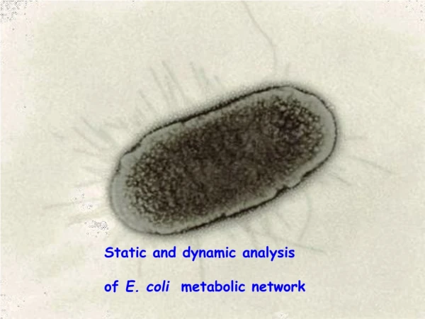
Dive into the complex metabolic pathways of E. coli using computational approaches for understanding causality and behavior at a system level. Static network analysis tracks causality, while dynamic models delve into metabolic control and flux analysis. Learn how researchers tackle biological problems in silico.

E N D
Static and dynamic analysis of E. coli metabolic network
Biochemical pathway: Network of biochemical reactions i.e. metabolites (nodes) “connected” by reactions Note: In living organisms biochemical reactios are (almost) always catalyzed by enzymes
Biochemical pathways are usually classified according to their “role”: Signaling pathways Gene regulatory networks Metabolic Pathways We focus on
Cellular metabolic pathways: complex networks of interactions Various kind of components: Metabolites; Proteins; Inorganic ions. Various kind of interaction Direct “causation”; +/- feedbacks. Complex, non linear dynamic behaviour e.g. glycolytic oscillations.
Computational approaches help in investigating the role played by single components in the behaviour at the system level
Computational approaches: Amount of details required Computational power required Interest of many computer scientists Dynamical models: Deterministic Metabolic Control Analysis Metabolic Flux Analysis Stochastic Process calculi based Flux balance analysis: Static network analysis: Pathway logic (Talcott et al. 2002) Biocham (Fages et al.2005) CP(Graph) (Dooms et al. 2000) Palsson et al. since 1995
What biologists (usually) want: Solve biological problems: Organize existing information; Accommodate new information in a coherent framework; Gain knowledge about systems (predict behaviour in silico); Drive wet lab experiments (pruning of hypotheses); ……… (Not necessarily biologists need fully detailed models!)
Different approaches towards satisfying biologist needs: Amount of details required Computational power requested Interest of computer scientists Dynamical models: Deterministic Stochastic Flux balance analysis: Static network analysis:
Both approaches focus on the same real organism: E.Coli K12 Genome of 4.7x10⁶ bp, including ~ 3200 genes The analysed network: Genome-scale metabolic model (Palsson et al., 2005) including 904 genes
Static network analysis approach: tracking causality in metabolic networks Chiara Bodei Davide Chiarugi Andrea Bracciali
Determining causal relationships could be non trivial in metabolic networks, e.g.: A B Does A contribute to cause (produce) B ? What happens ifA is removed from the system ?
Our approach: Askeletal description language to abstractly specify the clearly understood causal relations amongst the elements composing the network. Tailored simplifications: we are interested in causality only!! In describing biochemical reactions, we abstract away from: quantities, temperature …….; stoichiometric proportions; kinetic or thermodynamics parameters; and the dynamical evolution of reactions i.e. we project reactions on a “flat” temporal scale: reactants are not consumed by reactions. This approximated model allow us to effectively perform causality analysis
[ APPROACH ] Consider a (bio) chemical reaction, in the classical notation: aA + bB cC + dD Where: A and B are the reactants, C and D the products and a,b,c,d the Stoichiometric parameters. Under our approximation we obtain: A ○ B C ○ D We call it a rule: the presence of both A and B represents the possibility for C and D to be produced or caused. More precisely, the meaning of this epression would be as: A + B A + B + C + D We do not consider the dynamic evolution and, therefore, we do not describe reactants consumption
[ APPROACH ] The description of causal relationships within a metabolic network can be madebydefining: a set of reaction rules R, as described before, that describe how new metabolites can be produced. a set I of the metabolites initially present in the experiment Example: The upper part of glycolysis Reaction rules (R) glc6p fru6p fru6p ° ATP fru16p ° ADP fru16p ° gap dhap dhap gap gap dhap gap ° nad bpg13 ° nadh Initial state (I) tglc6p ATP nad
[ APPROACH ] Intuitively, given the set R and the set I, we define an explanation for a given metabolite a, the chain of rules that, starting from an (element of) I, leads to a. The existence of an explanation for a gives us indications on the possibility of the production of a. Note that Up to the adequacy of the adopted biological model, the lack of an explanation for a given metabolite represent a strong evidence of the impossibility for that metabolite to be produced in the real case.
[ The computational framework] Causal rules, as described, have a straightforward logical interpretation. More specifically, they can be directly translated into Horn Clauses (rules as clauses, and elements in the initial states as facts). A bottom-up semantics allows us to constructively determine the set of reactants that can be produced by the network: Starting from the set of facts I, rules in R are repeatedly applied [i.e. the consequences of the rules whose premises belongs to the set of the possbily produced reactant are added to the set itself] until they are ableto causethe possibility of new reactants. Under the working hypotheses, the process finitely converges to a finite set. The process is correct: a reactant belongs to the computed set iff an explanation for it exists
[ IN SILICO EXPERIMENTATION ] In silico gene KO applying the what-if strategy: What happens if a gene coding for an enzyme (and so the enzyme itself) involved in a metabolic network is silenced ? Test set: the metabolic network of E-coli k-12by Palsson and co-workers ( about 600 bio chemical reactions) Our toolkit allows straightforward, one-shot gene KO simulations : :- remove [Rule] removes the reaction(s) catalyzed by the enzime (simulates gene KO) :-Add [Rule] allows to compositionally expand the network :- Check[metabolite] check whether a metabolite has an explanation We typicaly obtain an answer in a wink !
[ IN SILICO EXPERIMENTATION ] What is the price we chose to pay for efficiency ? Recall the approximation: A ○ B C ○ D ~ A + B + C + D (no reactant consumption) This is a heavy approximation of reality: metabolites result producible disregarding the actual availability of reactants But allows to perform quick responsive and reiterable what-if experiments
[ IN SILICO EXPERIMENTATION – I ] Mutually essential genes for succinyl-CoA production: Genes sucAB (alpha-ketoglutarate dehydrogenase) and sucCD (succinyl-CoA synthase) of E. coli k-12 could be knocked-outindividually, but notsimultaneously to achieve Succinyl-CoA production. In silico KO: We removed the rules corresponding to the reactions catalyzed by the target enzymes; Outcome: Succinyl-CoA was not produced in silico (i.e. there was no explanation for Succinyl-CoA) only when both the target genes (i.e. the rules corresponding to the action of the encoded enzyme) were simultaneously turned off.
[ IN SILICO EXPERIMENTATION - II ] Essential genes for cellular life Extensive in silico gene KO experiments, to test gene essentiality i.e. verifying whether or not in silico knock-out mutants exhibit features typical of living cells: These characteristics could reasonably include: the production of ATP (essential for cellular energetic metabolism); the production of reduced coenzymes NADPH and NADH; structural components, such as the cell wall (murein Biosynthesis). Sample of 114 genesof our set. For each gene: - We removed the rule(s) corresponding to the reaction catalysed by the encoded enzyme - We checked for the presence of the observed elements at the end of each computation. We compared our results with the information contained in the “Geno Base”
[ IN SILICO EXPERIMENTATION ] ACCURACY: A = (TP + TN)/(TP + TN + FP + FN) Where: FP false positives, (the mutant is predicted unviable, but actually lives) FN false negatives (the mutant is predicted viable, but actually it is not), TP true positives (both in silico and in vivo mutants are viable) TN true negatives (both in silico and in vivo mutants are not viable) Our accuracy : 81% Other methods: 60% to 74% (Synthetic accessibility) 62% to 86% (Flux balance analysis, Palsson et al. )
Dynamical stochastic approach: tracking dynamical behaviours of whole-cell scale metabolic model Davide Chiarugi Pierpaolo Degano Jan Van Klinken Roberto Marangoni
The target biological system: E.Coli K12 The main goal: addressing network dynamics in a whole cell model The analysed network: Genome-scale metabolic model (Palsson et al., 2005) including 904 genes
The formalism: a specially tailored subset of π-calculus No restriction Name passing actually not used (synchronization only) Link with biological parameters: Gibbs free energy Activation energy
Example: aldolase Dihydroxyacetone-phosphate + D-Glyceraldehyde-3Pβ-D-Fructose 1-6bP becomes product Reactants channel Dihydroxyacetone-phosphate D-Glyceraldehyde-3-P .β-D-Fructose 1-6bP .0 = aldolase<a> = aldolase(x) Formal description of E.coli K12 genome-scale metabolic model (~ 850 reactions and ~ 700 metabolites)
In silico esperimentation Please wait next part of the talk (Jan) for details about the used toolkit ! Experimental starting conditions: Mimick continuous cultures; User defined initial quantities of metabolites Virtual experiments: Computations of about 107transitions each
Results: • Time course of metabolites concentration reaches the steady-state (homeostasys) as confirmed by regression analysis; Relative quantities of virtual key metabolites ~ real ones:
In silico gene KOs: studying re-routing of metabolic fluxes after gene deletions ppc KO (pep carboxylase) Anaerobiosis, glucose-limited pgi (phosphoglucose isomerase) zwf (glucose-6-P dehydrogenase) Ammonia or glucose-limited
Like in real prokaryotes! Results obtained in other works1: Analysis of complex dynamical behaviours glycolytic oscillations When glucose is continuously fed, sustained oscillations emerge…. 1. D. Chiarugi, M. Chinellato, P.Degano, G. Lo Brutto R. Marangoni, CMSB 2006