Download
1 / 41
410 likes | 428 Views
“Gradient Setup Techniques” Professor: - Dr Ajay Gupta Presented By: -vivek Kinra CS691 Spring 2003 Source: - http://www.cs.ucla.edu/classes/fall01/cs218/l1/project/student/ http://lecs.cs.ucla.edu/~estrin/talks. Recap. Characteristics of a Sensor Network:

E N D
“Gradient Setup Techniques” Professor: - Dr Ajay Gupta Presented By: -vivek Kinra CS691 Spring 2003 Source: -http://www.cs.ucla.edu/classes/fall01/cs218/l1/project/student/ http://lecs.cs.ucla.edu/~estrin/talks vivek CS-WMU
Recap • Characteristics of a Sensor Network: • Data centric: sensors are addressed by interests expressed by user queries • Scalable: no sensor has complete knowledge of the whole system • Energy-sensitive: sensors have limited battery power • Data dissemination is application-specific: data paths are determined by the needs of the application using the data • Adaptive: path selection may change as the energy level of certain paths decrease with use vivek CS-WMU
Recap contd • Sink->Generate Interest->Propagate Interest throughout N/W. • Sensor with that info (SOURCE) ->respond ->collecting required info->forwarding it back towards sink. • User addresses entire N/W with there quires instead of global addressing scheme vivek CS-WMU
contd • Naming • Gradient Setup • Reinforcement (When, Whom, How Many, Negative reinforcement) vivek CS-WMU
Sending data Source Sink Reinforcing stable path Source Source Sink Sink Recovering from node failure Illustrating Directed Diffusion Setting up gradients Source Sink vivek CS-WMU
Interest Propagation Setting up gradients Source Sink vivek CS-WMU
contd • I-P also becomes G establishment • Each node become sink for propagating interest to its neighbor • Receiving path becomes sending path • Upon receiving interest from a neighbor, an intermediate node will create a gradient for the link in reverse direction back to its neighbor vivek CS-WMU
contd • Interest Message may specify the loc of target query (x=10, y=4) • Non spatial interest are more vague and may require more flooding • Single Sink Case • User identification, • initiation time, • max hop count, localized identification on the one previous hop away vivek CS-WMU
Interest Propagation Steps • 1st time: -node will record interest and calculate gradient for the reverse path of the link to its neighbor (previous hop) • Based on gradient just established, the sensor can determine if the reverse path likely to carry data back to the sink • Hop count > 0 and intermediate sensor decrease hop count and forwards interest • Sensor doesn’t forward interest twice vivek CS-WMU
contd • Intermediate sensors must forward the data along the link with the greatest gradient and decide whether to forward it to other links that may have a comparable tendency to reach the sink • The source tags each piece of data with a timestamp so that intermediate nodes will drop duplicate data and prevent a data-forwarding loop • Finally if the node can obtain the data in query, it becomes the source node and sent back the collected data. • Multiple Sink Case vivek CS-WMU
Gradient • G in N/W shape the data routing paths to that network • Also G establishment is determined by application req, diff paths may be established for same data • Data aggregation->data propagation more efficient. Multiple (sink or source) • Energy awareness vivek CS-WMU
Schemes • Direction-based Scheme (COS) • Data is directed towards the sink in a straight line with as little deviation as possible • Each sensor knows its relative position • The interest message includes the sink’s position and the position of the previous hop neighbor vivek CS-WMU
contd • The gradient can be given by the function cos • The gradient = 0 when = 90 (when snb is perpendicular to ssink) • The gradient > 0 when < 90 • The gradient < 0 when > 90 (a negative gradient discourages data forwarding along that link) cos nb s neighbor source Sink vivek CS-WMU
Distance-based Scheme (ttl) • Data is directed towards the sink along the shortest path • The interest message contains a maximum hop count that each intermediate sensor decreases as it forwards • Based on this hop count, a node can determine its neighbor’s distance to the sink vivek CS-WMU
contd • Distance-based gradient is determined by 1/(ttl+1) • (ttl+1) is used because ttl = 0 when nb is exactly the sink • Distance-based gradient is the inverse of hop count 1/(ttl+1) nb s ttl hops sink source vivek CS-WMU
Gravity based Treat data forwarding like gravitational attraction where the sink exerts a gravity that is inversely proportional to the hop count Gradients are calculated by cos/(ttl+1)2 The gravity-based gradient is a combination of the distance and direction gradients cos /(ttl+1)2 nb s source sink vivek CS-WMU
(2, 6) (2, 7) (2, 5) (0, 4) (2, 4) (2, 3) (0, 2) (2, 2) A sensor node (2, 1) (2, 0) A sample topology vivek CS-WMU
0 0.707 1 1 1 1 Data flow A link 1 0.894 A source node 1 A sink node 1 A sensor node 1 Data flow with direction-based gradient vivek CS-WMU
1/2 1/3 1/6 1 1/5 1/2 1/4 Data flow A link 1/3 A source node 1/2 A sink node 1 A sensor node 1 Data flow with distance-based gradient vivek CS-WMU
0 .079 .028 1 0.04 0.224 0.063 Data flow A link 0.111 A source node 0.25 A sink node 1 A sensor node 1 Data flow with gravity-based gradient vivek CS-WMU
Energy Awareness • Consider Energy consumption level w/ gradient • If same gradient but different energy, choose higher energy • 2 Goals: • Each sensor minimize energy consumption • Even out energy dissipation in entire network • Energy Watermark determines when to consider minimizing energy vivek CS-WMU
contd • If sensor overused and has lower energy compared to other neighbors then link should be assigned a lower gradient to decrease the chance it will used again • Sensor maintains up-to-date energy info of all its neighbors. • Inefficient vivek CS-WMU
Data Aggregation • Duplicate interests to node from same link • Save energy by eliminating duplicate packets • Goal: Send data on link which best satisfies all interests vivek CS-WMU
Experiments • 3 schemes ( COS, TTL, Gravity) • Total Energy Consumption • Success Ratio (delivery of packets) • Data Aggregation • Average energy consumption at each node vivek CS-WMU
Experimental Setup – Energy Consumption • 10 random topologies (64 x 64) • 7% sensor density in the network • 3 schemes with/without Energy Awareness • Guarantee 100% success ratio • 99.9% Confidence Intervals • Long Hop (7-10 hops) • Short Hop (3-4 hops) vivek CS-WMU
contd • Each sensor has transmitting range of 8 units in the area • Sensor uses :- • Size of message • Energy units to transmit an interest • Size of message energy units for data propagation vivek CS-WMU
Ave Number of Hops:Long Hop vivek CS-WMU
Experimental Setup – Aggregation • 1 random topology (64x64) • 6.9% sensor density in the network • 3 different positions • 3 schemes with/without Energy Awareness U2 U2 S S S U2 U1 U1 U1 vivek CS-WMU
Aggregation – Energy Consumption vivek CS-WMU
Conclusion • Gravity Scheme uses less Energy, but unreliable when multiple users in different directions • Energy Awareness doesn’t improve the evenness of consumption per node vivek CS-WMU
Naming schemes • Internet where IP address provides low level names for routing • Web and the search engines provide document and object naming scheme • We need naming scheme that doesn’t relay on network topologies • Rather we need low level communication based on names that are external to N/W topologies vivek CS-WMU
contd • We need application relevant or it can be based on sensor types or geographic locations • Attribute based naming system vivek CS-WMU
Tiny Diffusion • Implementation of Diffusion on resource constrained USB motes • 8 bit CPU, 8k program memory, 512 bytes data memory • Subsets of full system • Retains only gradients and condenses attributes to a single tag • Entire system runs for less than 5.5 KB memory vivek CS-WMU
contd • Tiny OS adds ~3.5 KB and 144 bytes of data (inclusive support for radio and photo sensor • Diffusion adds ~2k code and 110 bytes of data to tiny OS vivek CS-WMU
Tiny Diffusion Functionality • Resource Constraint • Limited Cache size-currently 10 entries of 2 bytes each • Limited ability to support multiple traffic stream. currently support 5 concurrently active gradients vivek CS-WMU
TinyDiffusion Architecture vivek CS-WMU
Description • Fig shows interconnects b/n Filters, TinyDiffusion, AM, Timers and the photo components • Filters connected -> diff ports of the Timers which export alarms for periodic events • SRC is connected to both 0 and 1 port of Timers vivek CS-WMU
conts • Filters connect at different ports to the TinyDiffusion to send and receive packets. • They specify which attribute types they are interested in AND when the attribute type in packed matches the specified type, the packed is sent to the corresponding filter. • Active Messaging layer vivek CS-WMU
RFM Acoustic Data Source Query Data Sink Transceiver DIFFUSION Device Driver TINYOS LINUX Photo Data Source Data Sink TinyDiffusion TINYOS Gateway Architecture MOTE ATMEL 8586 4MHz MCU 8K program memory 512 Bytes Data Memory RFM Radio 900 MHz PC104 AMD Elan™SC400 66MHz CPU 16MB RAM Form Factor: 3.6" x 3.8" x 0.6" vivek CS-WMU
Tiered Testbed • PC-104+(linux) with MoteNIC • Tags, Sensor Card • UCB Motes w/TinyOS • Yet to come: SmartDust (highly specialized nodes) PC104 TAG USB Mote vivek CS-WMU