Download

1 / 32
330 likes | 359 Views
Learn about removing internal and external noise from heart sounds using Independent Component Analysis (ICA) to improve monitoring accuracy. Explore the principles, computations, and experimental results of this innovative method.

E N D
Heart Sound Background Noise Removal Haim Appleboim Biomedical Seminar February 2007
Overview • Current cardiac monitoring relies on EKG • EKG provides full information about the electrical activity but very little information about the mechanical activity • Echo provides full info about the mechanical activity • Echo can not be used for continuous monitoring • Heart Sounds may provide information about mechanical activity
Overview • Monitoring heart sounds continuously in non clinical environment is difficult due to background sounds and noise both externally and internally • This work introduces a method for removal of internal (and external) background sound such as speech (of the patient)
Overview • Heart Sounds are vulnerable to sounds created by the monitored person due to significant overlap in frequency with speech • Thus, filters are less effective in removing the noise
A novel approach based on ICA • ICA: Independent component analysis is a general method for blind source separation. • It has not been used in the context of heart background sound removal • We shall demonstrate its superiority over other methods.
Sound A S1 Sm-1 Sound B Sm Sound C ICA (Independent Component Analysis) x = As Each sensor receives a linear mixture of all the signal sources It is required to determine the source signals
ICA definition • ICA of a random vector X consists of estimating the following generative model for the data: • The independent components are latent variables They cannot be directly observed • The independent components are assumed to have a non-Gaussian distributions • The mixing matrix is assumed to be unknown • All we observe is the general vector x and we must estimate both A and s using it
Independent Components Computation • After estimating the mixing matrix A we can de-mix by computing it’s inverse: • Then we obtain the independent components (de-mix) simply by:
Principles of ICA Estimation • The fundamental restriction in ICA is that the fundamental components must be non-Gaussian for ICA to be possible • The Linear combination of independent variables is more Gaussian than each of the variables • To estimate one of the Independent components y let us write: • W is One of the rows of A-1 and should be estimated • Linear combination of independent variables is more Gaussian than each of the variables zTs is more Gaussian than each of the Si The minimal gaussianity is achieved when it equals to one of the Si • We can say that W is a vector which maximizes the nongaussianity of WTX (one of the Independent Components)
FastICA (Hyvärinen, Oja) • FastICA learning finds a direction: unit vector w, such that the projection wTx maximizes non-Gaussianity • FastICA for one unit computational steps: • Choose an initial weight vector • If w did not converge go back to 2 • FastICA for several units • To estimate several independent components the one unit algorithm must run using several units with weight vectors • To prevent different vectors converging to the same maxima, after each iteration the outputs must be de-correlated
Spectral ICA • Spectral ICA: performing ICA on a frequency domain signal (Problem when the Spectrum is complex) • Solved using DCT (Discreet Cosine Transform) • Spectral ICA algorithmic flow • Perform DCT on the input data • Run FastICA on data after DCT • Perform Inverse DCT
Spectral ICA: Why doe’s it work better? • Spectral ICA attempts to separate each frequency component from different sources (ignoring the delays) • Since the background sound has overlapping spectrum with the HS but with different magnitudes in each channel, it should be easier to separate and remove
Algorithm Quality assessment • Quality assessment methods • “Human eye” assessment • Algorithmic assessment • FFT plots • Spectrogram plots • Diastole Analysis (Noise Removal Quality) • Diastole Analysis calculation steps: • A = ICA Diastole Peaks average • B = NoisySig Diastole Peaks average • Noise Removal Quality = B / A
Result with Spectral ICA (1) Time Domain HS file name used in this example is ‘GA_Halt_1’, ICA type is ‘Gauss’, Noise file is ‘count_time’
Result with Spectral ICA (2) Time Domain HS file name used in this example is ‘GA_Halt_1’, ICA type is ‘Gauss’, Noise file is ‘television’ Spectral Domain
FastICA FastICA Wiener Filter Wiener Filter Wiener Filter FastICA Result with Spectral ICA (3) Diastole (Quite period) analysis results HS file name used in this example is ‘GA_Halt_1’, Noise file name used is ‘snor_with_pre’ and FastICA type is ‘Gauss’
Cases when ICA doesn't work well Unsuccessful noise removal attempt for a HS with a peak noise caused by microphone movement HS file name used in this example is ‘GA_Halt_1’, FastICA type is ‘Gauss’, Noise file is ‘count_time’
Spectral ICA Time ICA Spectral ICA Time ICA Time vs. Spectral ICA (1) HS file name used in this example is ‘Halt_Supine_1’, Noise file is ‘count_time, FastICA type is ‘Gauss’
Spectral ICA Time FastICA Spectral ICA Time ICA Time vs. Spectral ICA (2) HS file name used in this example is ‘GA_Halt_1’, Noise file name used is ‘snor_with_pre’ and FastICA type is ‘Gauss’
ICA nonlinearity = pow3 ICA nonlinearity = tanh ICA nonlinearity = Gauss ICA nonlinearity = skew Results vs. Nonlinearity HS file name used in this example is ‘GA_Normal_1’, Noise file is ‘count_time’
Real Noisy Environment Results HS file name used in this example is ‘HAIM_COUNT_1’, FastICA type is ‘Gauss’
Summery • we have introduced a practical method for background noise removal in heart sounds for the purpose of continues heart sounds monitoring • The superiority of the proposed method over conventional ones makes it into a practical way of providing high quality heart sound in a noisy environment
Principles of ICA Estimation (Measures of nongaussianity) • Measures of nongaussianity • Kurtosis • Negentropy • Minimization of mutual information
Kurtosis • Kurt (y) = E{y4} – 3(E{y2})2 • E{y2} = 1 Kurt (y) = E{y4} – 3 • Y Gaussian E{y4} = 3(E{y2})2 Kurt (y) = 0 ↓ • Therefore kurtosis is 0 for a Gaussian random variable. • For most Nongaussian random variables kurtosis ≠ 0 • kurtosis can be both positive or negative. • Typically nongaussianity is measured by the absolute value of kurtosis.
Negentropy • The entropy of a random variable is the degree of information that an observation of the variable gives. Entropy is related to the coding length of the random variable. • The more random the variable is, the larger is it’s entropy. • For a discrete random variable entropy is defined as: H(Y) = -Σ P(Y=ai) · log P(Y=ai) • Gaussian variable has the largest entropy among all random variables of equal variance therefore , entropy can be used as a measure of nongaussianity.
Negentropy • For a continues random variable differential entropy is defined as: H(y) = -∫f(y)·log(f(y))·dy • Negentropy (modified version of differential entropy) is defined as: J(y) = H(ygauss) – H(y) • According to the above definition Negentropy is always non-negative and is zero if and only if y has Gaussian distribution.
Negentropy • Practically the estimation of NEGENTROPY is rather difficult. Therefore we usually us some approximations for this purpose
Principles of ICA Estimation(Minimization of mutual information) • Definition of mutual information I between m random variables: I(y1,y2, …,ym) = Σ H(yi)-H(y) • Mutual Information is a measure of dependence between random variables. • It is always non negative and zero if and only if the variables are statistically independent. • For an invertible linear transformation y=Wx we can write: I(y1,y2,…) = Σ H(yi)-H(x)-log|det(w)| I(y1,y2,…) = Σ C-J(yi)
Principles of ICA Estimation(Minimization of mutual information) • Finding the invertible transformation W that minimizes the mutual information is equivalent to fining the direction in which the negentropy J is maximized.