Download
1 / 46
460 likes | 478 Views
Learn about Convex Hull algorithms for point sets in computational geometry. Explore Gift Wrapping, Incremental Insertion, and Divide & Conquer methods. Understand convexity, representation, and testing of convex hulls. Discover the algorithms, principles, and complexities involved in these computations.

E N D
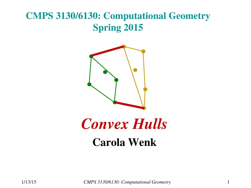
CMPS 3130/6130: Computational GeometrySpring 2015 Convex Hulls Carola Wenk CMPS 3130/6130: Computational Geometry
Convex Hull Problem • Given a set of pins on a pinboard and a rubber band around them. How does the rubber band look when it snaps tight? • The convex hull of a point set is one of the simplest shape approximations for a set of points. CMPS 3130/6130: Computational Geometry
Convexity • A set C R2 is convex if for every two points p,qC the line segment pq is fully contained in C. convex non-convex CMPS 3130/6130: Computational Geometry
Convex Hull • The convex hull CH(P) of a point set P R2 is the smallest convex set C P. In other words CH(P) = C . C PC convex P CMPS 3130/6130: Computational Geometry
4 5 3 6 2 1 0 Convex Hull • Observation: CH(P) is the unique convex polygon whose vertices are points of P and which contains all points of P. • Goal: Compute CH(P). What does that mean? How do we represent/store CH(P)? Represent the convex hull as the sequence of points on the convex hull polygon (the boundary of the convex hull), in counter-clockwise order. CMPS 3130/6130: Computational Geometry
A First Try Algorithm SLOW_CH(P): /* CH(P) = Intersection of all half-planes that are defined by the directed line through ordered pairs of points in P and that have all remaining points of P on their left */ Input: Point set P R2 Output: A list L of vertices describing the CH(P) in counter-clockwise order E:= for all (p,q)PP with p≠q // ordered pair valid := true for all rP, r≠p and r≠q if r lies to the right of directed line through p and q// takes constant time valid := false if valid then E:=Epq// directed edge Construct from E sorted list L of vertices of CH(P) in counter-clockwise order • Runtime: O(n3) , where n = |P| • How to test that a point lies to the right of a directed line? CMPS 3130/6130: Computational Geometry
Orientation Test / Halfplane Test p r q q r q r p p • negative orientation (clockwise) • r lies to the right of pq • positive orientation(counter-clockwise) • r lies to the left of pq • zero orientation • r lies on the line pq 1 px py1 qx qy1 rx ry • Orient(p,q,r) = sign det • Can be computed in constant time ,where p = (px,py) CMPS 3130/6130: Computational Geometry
Jarvis’ March (Gift Wrapping) AlgorithmGiftwrapping_CH(P): // Compute CH(P) by incrementally inserting points from left to right Input: Point set P R2 Output: List q1, q2,… of vertices in counter-clockwise order around CH(P) q1 = point in Pwith smallest y (if ties, with smallest x) q2 = point in P with smallest angle to horizontal line through q1 i = 2 do { i++ qi = point with smallest angle to line through qi-2 and qi-1 } while qi ≠q1 q3 q2 q1 • Runtime: O(hn) , where n = |P| and h = #points on CH(P) • Output-sensitive algorithm CMPS 3130/6130: Computational Geometry
Incremental Insertion AlgorithmIncremental_CH(P): // Compute CH(P) by incrementally inserting points from left to right Input: Point set P R2 Output:C=CH(P), described as a list of vertices in counter-clockwise order Sort points in P lexicographically (by x-coordinate, break ties by y-coordinate) Remove first three points from P and insert them into C in counter-clockwise order around the triangle described by them. for all pP// Incrementally add p to hull Compute the two tangents to p and C Remove enclosed non-hull points from C, and insert p O(n log n) O(1) n-3 times O(i) O(i) n • Runtime: O(i) = O(n2) , where n = |P| i=3 • Really? CMPS 3130/6130: Computational Geometry
Tangent computation vt succ(pi-1) pi-1 pi pred(pi-1) vb upper_tangent(C,pi): // Compute upper tangent to pi and C. Return tangent vertex vt vt = pi-1 while succ(vt) lies above line through pi and vt vt = succ(vt) returnvt Amortization: Every vertex that is checked during tangent computation is afterwards deleted from the current convex hull C CMPS 3130/6130: Computational Geometry
Incremental Insertion AlgorithmIncremental_CH(P): // Compute CH(P) by incrementally inserting points from left to right Input: Point set P R2 Output:C=CH(P), described as a list of vertices in counter-clockwise order Sort points in P lexicographically (by x-coordinate, break ties by y-coordinate) Remove first three points from P and insert them into C in counter-clockwise order around the triangle described by them. for all pP// Incrementally add p to hull Compute the two tangents to p and C Remove enclosed non-hull points from C, and insert p O(n log n) O(1) n-3 times O(1) amort. O(1) amort. • Runtime: O(n log n + n)= O(n log n), where n = |P| CMPS 3130/6130: Computational Geometry
A B Convex Hull: Divide & Conquer • Preprocessing: sort the points by x-coordinate • Divide the set of points into two sets A and B: • A contains the left n/2 points, • B contains the right n/2 points • Recursively compute the convex hull of A • Recursively compute the convex hull of B • Merge the two convex hulls CMPS 3130/6130: Computational Geometry
Merging • Find upper and lower tangent • With those tangents the convex hull of AB can be computed from the convex hulls of A and the convex hull of B in O(n) linear time A B CMPS 3130/6130: Computational Geometry
left turn right turn check with orientation test Finding the lower tangent 3 a = rightmost point of A b = leftmost point of B while T=ab not lower tangent to both convex hulls of A and B do{ while T not lower tangent to convex hull of A do{ a=a-1 } while T not lower tangent to convex hull of B do{ b=b+1 } } 4=b 4 2 3 5 5 a=2 6 1 7 1 0 0 A B CMPS 3130/6130: Computational Geometry
Convex Hull: Runtime O(n log n) just once • Preprocessing: sort the points by x-coordinate • Divide the set of points into two sets A and B: • A contains the left n/2 points, • B contains the right n/2 points • Recursively compute the convex hull of A • Recursively compute the convex hull of B • Merge the two convex hulls O(1) T(n/2) T(n/2) O(n) CMPS 3130/6130: Computational Geometry
Convex Hull: Runtime • RuntimeRecurrence: T(n) = 2 T(n/2) + cn • Solves to T(n) = (n log n) CMPS 3130/6130: Computational Geometry
Recurrence (Just like merge sort recurrence) • Divide: Divide set of points in half. • Conquer: Recursively compute convex hulls of 2 halves. • Combine: Linear-time merge. T(n) = 2T(n/2) + O(n) work dividing and combining # subproblems subproblem size CMPS 3130/6130: Computational Geometry
T(n) = Q(1)ifn = 1; 2T(n/2) + Q(n)ifn > 1. Recurrence (cont’d) • How do we solve T(n)? I.e., how do we find out if it is O(n) or O(n2) or …? CMPS 3130/6130: Computational Geometry
Recursion tree Solve T(n) = 2T(n/2) + dn, where d > 0 is constant. CMPS 3130/6130: Computational Geometry
Recursion tree Solve T(n) = 2T(n/2) + dn, where d > 0 is constant. T(n) CMPS 3130/6130: Computational Geometry
dn T(n/2) T(n/2) Recursion tree Solve T(n) = 2T(n/2) + dn, where d > 0 is constant. CMPS 3130/6130: Computational Geometry
dn dn/2 dn/2 T(n/4) T(n/4) T(n/4) T(n/4) Recursion tree Solve T(n) = 2T(n/2) + dn, where d > 0 is constant. CMPS 3130/6130: Computational Geometry
Recursion tree Solve T(n) = 2T(n/2) + dn, where d > 0 is constant. dn dn/2 dn/2 dn/4 dn/4 dn/4 dn/4 … Q(1) CMPS 3130/6130: Computational Geometry
Recursion tree Solve T(n) = 2T(n/2) + dn, where d > 0 is constant. dn dn/2 dn/2 h = log n dn/4 dn/4 dn/4 dn/4 … Q(1) CMPS 3130/6130: Computational Geometry
Recursion tree Solve T(n) = 2T(n/2) + dn, where d > 0 is constant. dn dn dn/2 dn/2 h = log n dn/4 dn/4 dn/4 dn/4 … Q(1) CMPS 3130/6130: Computational Geometry
Recursion tree Solve T(n) = 2T(n/2) + dn, where d > 0 is constant. dn dn dn/2 dn dn/2 h = log n dn/4 dn/4 dn/4 dn/4 … Q(1) CMPS 3130/6130: Computational Geometry
Recursion tree Solve T(n) = 2T(n/2) + dn, where d > 0 is constant. dn dn dn/2 dn dn/2 h = log n dn/4 dn/4 dn dn/4 dn/4 … … Q(1) CMPS 3130/6130: Computational Geometry
Recursion tree Solve T(n) = 2T(n/2) + dn, where d > 0 is constant. dn dn dn/2 dn dn/2 h = log n dn/4 dn/4 dn dn/4 dn/4 … … Q(1) #leaves = n Q(n) CMPS 3130/6130: Computational Geometry
Recursion tree Solve T(n) = 2T(n/2) + dn, where d > 0 is constant. dn dn dn/2 dn dn/2 h = log n dn/4 dn/4 dn dn/4 dn/4 … … Q(1) #leaves = n Q(n) Total Q(n log n) CMPS 3130/6130: Computational Geometry
The divide-and-conquer design paradigm • Divide the problem (instance) into subproblems. a subproblems, each of size n/b • Conquer the subproblems by solving them recursively. • Combine subproblem solutions. Runtime is f(n) CMPS 3130/6130: Computational Geometry
Master theorem T(n) = aT(n/b) + f(n) , where a³ 1, b > 1, and f is asymptotically positive. CASE 1:f(n) = O(nlogba – e) T(n) = Q(nlogba) . CASE 2:f(n) = Q(nlogba logkn) T(n) = Q(nlogba logk+1n) . CASE 3:f(n) = W(nlogba + e) and af(n/b) £cf(n) T(n) = Q(f(n)) . Convex hull:a = 2, b = 2 nlogba = n CASE 2 (k = 0) T(n) = Q(n log n) . CMPS 3130/6130: Computational Geometry
Graham’s Scan Another incremental algorithm • Compute solution by incrementally adding points • Add points in which order? • Sorted by x-coordinate • But convex hulls are cyclically ordered Split convex hull into upper and lower part upper convex hull UCH(P) lower convex hull LCH(P) CMPS 3130/6130: Computational Geometry
Graham’s LCH Algorithm Grahams_LCH(P): // Incrementally compute the lower convex hull of P Input: Point set P R2 Output: A list L of vertices describing LCH(P) in counter-clockwise order Sort P in increasing order by x-coordinate P = {p1,…,pn} L = {p2,p1} for i=3 to n while |L|>=2 and orientation(L.second(), L.first(), pi,) <= 0// no left turn delete first element from L Append pi to the front of L O(n log n) O(n) • Each element is appended only once, and hence only deleted at most once the for-loop takes O(n) time • O(n log n) time total CMPS 3130/6130: Computational Geometry
Lower Bound • Comparison-based sorting of n elements takesW(n log n) time. • How can we use this lower bound to show a lower bound for the computation of the convex hull of n points in R2? CMPS 3130/6130: Computational Geometry
Decision-tree model A decision tree models the execution of any comparison sorting algorithm: • One tree per input size n. • The tree contains all possible comparisons (= if-branches) that could be executed for any input of size n. • The tree contains all comparisons along all possible instruction traces (= control flows) for all inputs of size n. • For one input, only one path to a leaf is executed. • Running time = length of the path taken. • Worst-case running time = height of tree. CMPS 3130/6130: Computational Geometry
Decision-tree for insertion sort Sort áa1, a2, a3ñ a1a2a3 insert a2 a1:a2 j i ³ < insert a3 a2a1a3 a2:a3 a1:a3 insert a3 a1a2a3 j i ³ < ³ < j i a1a2a3 a2a1a3 a1:a3 a2:a3 a1a2a3 a2a1a3 j i j i < < ³ ³ a1a3a2 a3a1a2 a2a3a1 a3a2a1 Each internal node is labeled ai:aj for i, j Î {1, 2,…, n}. • The left subtree shows subsequent comparisons if ai< aj. • The right subtree shows subsequent comparisons if ai³aj. CMPS 3130/6130: Computational Geometry
Decision-tree for insertion sort Sort áa1, a2, a3ñ = <9,4,6> a1a2a3 insert a2 a1:a2 j i ³ < insert a3 a2a1a3 a2:a3 a1:a3 insert a3 a1a2a3 j i ³ < ³ < j i a1a2a3 a2a1a3 a1:a3 a2:a3 a1a2a3 a2a1a3 j i j i < < ³ ³ a1a3a2 a3a1a2 a2a3a1 a3a2a1 Each internal node is labeled ai:aj for i, j Î {1, 2,…, n}. • The left subtree shows subsequent comparisons if ai< aj. • The right subtree shows subsequent comparisons if ai³aj. CMPS 3130/6130: Computational Geometry
Decision-tree for insertion sort Sort áa1, a2, a3ñ = <9,4,6> a1a2a3 insert a2 a1:a2 j i 9 ³ 4 < insert a3 a2a1a3 a2:a3 a1:a3 insert a3 a1a2a3 j i ³ < ³ < j i a1a2a3 a2a1a3 a1:a3 a2:a3 a1a2a3 a2a1a3 j i j i < < ³ ³ a1a3a2 a3a1a2 a2a3a1 a3a2a1 Each internal node is labeled ai:aj for i, j Î {1, 2,…, n}. • The left subtree shows subsequent comparisons if ai< aj. • The right subtree shows subsequent comparisons if ai³aj. CMPS 3130/6130: Computational Geometry
Decision-tree for insertion sort Sort áa1, a2, a3ñ = <9,4,6> a1a2a3 insert a2 a1:a2 j i ³ < insert a3 a1:a3 a2a1a3 a2:a3 insert a3 a1a2a3 j i < ³ 9 ³ 6 < j i a1a2a3 a2a1a3 a1:a3 a2:a3 a1a2a3 a2a1a3 j i j i < < ³ ³ a1a3a2 a3a1a2 a2a3a1 a3a2a1 Each internal node is labeled ai:aj for i, j Î {1, 2,…, n}. • The left subtree shows subsequent comparisons if ai< aj. • The right subtree shows subsequent comparisons if ai³aj. CMPS 3130/6130: Computational Geometry
Decision-tree for insertion sort Sort áa1, a2, a3ñ = <9,4,6> a1a2a3 insert a2 a1:a2 j i ³ < insert a3 a2a1a3 a2:a3 a1:a3 insert a3 a1a2a3 j i ³ < ³ < j i a1a2a3 a2a1a3 a2:a3 a1:a3 a1a2a3 a2a1a3 j i j i < ³ 4 < 6 ³ a1a3a2 a3a1a2 a2a3a1 a3a2a1 Each internal node is labeled ai:aj for i, j Î {1, 2,…, n}. • The left subtree shows subsequent comparisons if ai< aj. • The right subtree shows subsequent comparisons if ai³aj. CMPS 3130/6130: Computational Geometry
Decision-tree for insertion sort Sort áa1, a2, a3ñ = <9,4,6> a1a2a3 insert a2 a1:a2 j i ³ < insert a3 a2a1a3 a2:a3 a1:a3 insert a3 a1a2a3 j i ³ < ³ < j i a1a2a3 a2a1a3 a1:a3 a2:a3 a1a2a3 a2a1a3 j i j i < < ³ ³ a2a3a1 a1a3a2 a3a1a2 a3a2a1 4<6 9 Each internal node is labeled ai:aj for i, j Î {1, 2,…, n}. • The left subtree shows subsequent comparisons if ai< aj. • The right subtree shows subsequent comparisons if ai³aj. CMPS 3130/6130: Computational Geometry
Decision-tree for insertion sort Sort áa1, a2, a3ñ = <9,4,6> a1a2a3 insert a2 a1:a2 j i ³ < insert a3 a2a1a3 a2:a3 a1:a3 insert a3 a1a2a3 j i ³ < ³ < j i a1a2a3 a2a1a3 a1:a3 a2:a3 a1a2a3 a2a1a3 j i j i < < ³ ³ a2a3a1 a1a3a2 a3a1a2 a3a2a1 4<6 9 Each leaf contains a permutation áp(1), p(2),…, p(n)ñ to indicate that the ordering ap(1) £ap(2)£ ...£ap(n)has been established. CMPS 3130/6130: Computational Geometry
h ³ log(n!) (log is mono. increasing) ³ log ((n/2)n/2) = n/2 log n/2 h W(n log n). Lower bound for comparison sorting Theorem. Any decision tree that can sort n elements must have height W(nlogn). Proof. The tree must contain ³n! leaves, since there are n! possible permutations. A height-h binary tree has 2h leaves. Thus, n! 2h. CMPS 3130/6130: Computational Geometry
Lower Bound • Comparison-based sorting of n elements takesW(n log n) time. • How can we use this lower bound to show a lower bound for the computation of the convex hull of n points in R2? • Devise a sorting algorithm which uses the convex hull and otherwise only linear-time operations Since this is a comparison-based sorting algorithm, the lower bound W(n log n) applies Since all other operations need linear time, the convex hull algorithm has to take W(n log n) time CMPS 3130/6130: Computational Geometry
CH_Sort s2 Algorithm CH_Sort(S): /* Sorts a set of numbers using a convex hullalgorithm. Converts numbers to points, runs CH, converts back to sorted sequence. */ Input: Set of numbers S R Output: A list L of of numbers in S sorted in increasing order P= for each sS insert (s,s2) into P L’ = CH(P)// compute convex hull Find pointp’P with minimum x-coordinate for each p=(px,py)L’, starting with p’,add px into L return L s -2 -4 1 4 5 CMPS 3130/6130: Computational Geometry
Convex Hull Summary • Brute force algorithm: O(n3) • Jarvis’ march (gift wrapping): O(nh) • Incremental insertion: O(n log n) • Divide-and-conquer: O(n log n) • Graham’s scan: O(n log n) • Lower bound: (n log n) CMPS 3130/6130: Computational Geometry