Download
1 / 15
150 likes | 169 Views
This research focuses on forecasting gNL (non-Gaussianity) in the cosmic microwave background (CMB) for mixed isocurvature and adiabatic modes. The study explores different parameterizations and applies Planck data to estimate these parameters.

E N D
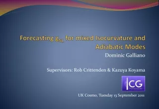
Forecasting gNL for mixed Isocurvature and Adiabatic Modes Dominic Galliano Supervisors: Rob Crittenden & Kazuya Koyama UK Cosmo, Tuesday 13 September 2011
Outline • Introduce four point statistics on the CMB. • Look at specific gNL terms for adiabatic case. • Look at gNL terms for mixed a mixed adiabatic and isocurvature case. • Introduce previous works defining new parameters. • Show Planck forecasts for new parameters. • Talk about current work.
Why measure non-Gaussianity? • Non Gaussianity helps discriminate between different inflation models. • Measured in the CMB though the temperature anisotropies: • The bispectrum measures non-Gaussianity, parameterised by an amplitude (e.g. fNLlocal) for a particular bispectrum shape. Previous parameter space
Why use the trispectrum? • The trispectrum provides independent information of non-Gaussianity, which require other parameterisations (e.g. gNL.). • It is possible for models to have a negligible bispectrum, but still have a significant trispectrum. This is the case with cosmic strings models. • As with the bispectrum there are different trispectrum shapes. gNL of the local type has been measured using WMAP data:-7.4 < gNL / 105 < 8.2 (Smidt et al. 1004.1409v2) -5.4 < gNL / 105 < 8.6 (Fergusson et al. 1012.6039v1)
Building the 4 Point Function • We take potential for the curvature perturbation in local form: • The Fourier transform of the curvature perturbation and the 4 point expectation value is calculated. The connected term of which is: • Tτ(k1,k2,k3,k4,k12,k14) contains the term built from the 1st order non linear term in (k).
Forming gNL terms • Tg(k1,k2,k3,k4) contain the terms built from the 2nd order correction in (k). • Remember we have: • Build trispectrum: k2 k1 k12 k3 k4
Mixing the modes • Recent work by Langlois and van Tent (arXiv: 1004.2567) have look at what happens when there are two different types of primordial modes. Specifically a single CDM isocurvature mode and the usual local adiabatic mode: • Two distinct transfer functions and two non-Gaussian sources, gave six different fnl shapes and eight different gnl shapes.
A Schematic • Simple model for modelling a non-Gaussian modes: • We can mixed these 5 different ways:
A Schematic • Simple model for modelling a non-Gaussian modes: • Choose one: There are two ways we can mix these • All these terms will have the following combination of transfer functions:
A Schematic • For a class of models one can normalise for a mixed power spectrum and an isocurvature power spectra:
Many parameters • Each is a different combination of transfer functions, power spectra of and S and fNLlocal and fNLS. These six shapes are parameterised by six new fNLparameters. • The forecast for these six parameters for Planck were derived using a Fisher Matrix. The bounds derived were: {10, 7, 143, 148, 166, 127}. • Previous work by Langlois and Takahashi (arXiv: 1012.4855) derived the shapes for the trispectrum. For the gNL type terms, there are eight different mixed shapes with eight new parameters.
Mixing the modes • In Langlois and Takahashi (arXiv: 1012.4855) they linked the non-Gaussian parameters to the theoretical parameters for a mixed curvaton and inflation model. • Applicable to any inflation theory with two different transfer function and two initial curvature perturbations. • Estimators can be constructed for each of these parameters.
Forecasting for Planck • Each Fisher matrix component is calculated using: Geometry Physics • Beam and noise are modelled on the first three HFI Planck channels. • Sum to = 1,000. • Code requires close to 13 hours on 408 cores. Planck will be sensitive to modes upto 2,500, and naïve scaling of this would require 4,750 CPU days to run.
Preliminary Trispectrum Results • Gives the following bounds: ∆gNLi / 1 E+06 = {3.3, 1.8, 1.4, 18, 37, 30, 15, 5.9}
Current Work • Sample the forecasts for > 1,000. • Apply bounds to specific inflation scenarios and their specific parameters. • Calculate forecasts for τNL terms. • Start work correlating estimators from different theories, such as the local gNL estimator and the equilateral gNL estimator.. • Correlation functions: