
Variogram Analysis: Parameters, Estimators, and Applications
E N D
Presentation Transcript
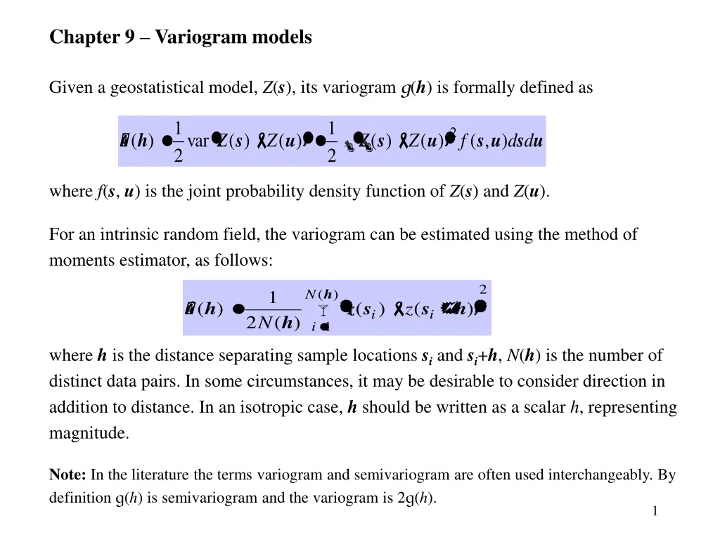
Chapter 9 – Variogram models Given a geostatistical model, Z(s), its variogram g(h) is formally defined as where f(s, u) is the joint probability density function of Z(s) and Z(u). For an intrinsic random field, the variogram can be estimated using the method of moments estimator, as follows: where h is the distance separating sample locations si and si+h, N(h) is the number of distinct data pairs. In some circumstances, it may be desirable to consider direction in addition to distance. In an isotropic case, h should be written as a scalar h, representing magnitude. Note: In the literature the terms variogram and semivariogram are often used interchangeably. By definition g(h) is semivariogram and the variogram is 2g(h).
Robust variogram estimator Variogram provides an important tool for describing how the spatial data are related with distance. As we have seen it is defined in terms of dissimilarity in data values between two locations separated by a distance h. It is noted that the moment estimator given in the previous page is sensitive to outliers in the data. Thus, sometimes robust estimators are used. The widely used robust estimator is given by Cressie and Hawkins (1980): The motivation behind this estimator is that for a Gaussian process, we have Based on the Box-Cox transformation, it is found that the fourth-root of 12 is more normally distributed. * Cressie, N. and Hawkins, D. M. 1980. Robust estimation of the variogram, I. Journal of the International Association for Mathematical Geology 12:115-125.
1.2 sill = 1.0 0.8 g(h) 0.4 nugget = 0.2 range h = 5 0.0 0 2 4 6 8 10 h Variogram parameters The main goal of a variogram analysis is to construct a variogram that best estimates the autocorrelation structure of the underlying stochastic process. A typical variogram can be described using three parameters: Nugget effect – represents micro-scale variation or measurement error. It is estimated from the empirical variogram at h= 0. Range – is the distance at which the variogram reaches the plateau, i.e., the distance (if any) at which data are no longer correlated. Sill – is the variance of the random field V(Z), disregarding the spatial structure. It is the plateau the variogram reaches at the range, g(range).
0.5 m 0.5 m 20° 5 m 20° • Setting variogram parameters • Construction of a variogram requires consideration of a few things: • An appropriate lag increment for h – It defines the distance at which the variogram is calculated. • A tolerance for the lag increment – It establishes distance bins for the lag increments to accommodate unevenly spaced observations. • The number of lags over which the variogram will be calculated – The number of lags in conjunction with the size of the lag increment will define the total distance over which a variogram is calculated. • A tolerance for angle – It determines how wide the bins will span. • Two practical rules: • It is recommended that h is chosen as such • that the number of pairs is greater than 30. • 2. The distance of reliability for an • experimental variogram is h < D/2, where • D is the maximum distance over the field of data.
Computing variograms An experimental variogram is calculated using the package geoR: Create a geodata data for Gigante soil data, surface water pH values: >soil87pH.geodat=as.geodata(soil87.dat,coords.col=2:3,data.col=5,covar.col=6:14) >variog.b=variog(soil87pH.geodat,max.dist=500) >variog.c=variog(soil87pH.geodat, max.dist=500, op=“cloud”) >plot(variog.b) >plot(variog.c)
Covariogram and Correlogram Covariogram (analogous to covariance) and correlogram (analogous to correlation coefficient) are another two useful methods for measuring spatial correlation. They describe similarity in values between two locations. Covariogram: Its estimator: where is the sample mean. At h = 0, Ĉ(0) is simply the finite variance of the random field. It is straightforward to establish the relationship: The correlogram is defined as
Properties of the moment estimator for variogram • It is unbiased: • If Z(s) is ergodic, as n . This means that the moment estimator approaches the true value for the variogram as the size of the region increases. The estimator is consistent. • The moment estimator converges in distribution to a normal distribution as n , i.e., it is approximately normally distributed for large samples. • For Gaussian processes, the approximate variance-covariance matrix of is available (Cressie 1985). • * Cressie, N. 1985. Fitting variogram models by weighted least squares. Mathematical Geology 17:563-586.
Properties of the moment estimator for covariance • The covariance: C(h) = cov(Z(si), Z(si+h)) • The moment estimator: • Properties: • The moment estimator for the covariance is biased. The bias arises because the covariance function for the residuals, is not the same as the covariance function for the errors, • For a second-order stationary random field, the moment estimator for the covariance is consistent: Ĉ(h)C(h) almost surely as n . However, the convergence is slower than the varigogram. • For a second-order stationary random field, the moment estimator is approximately normally distributed. • Properties 1 and 2 are the reasons why the variogram is preferred over the covariance function (and correlogram) in modeling geostatistical data.
g(h) h • Variogram models • There are two reasons we need to fit a model to the empirical variogram: • Spatial prediction (kriging) requires estimates of the variogram g(h) for those h’s which are not available in the data. • The empirical variogram cannot guarantee the variance of predicted values to be positive. A variogram model can ensure the variance positive. • Various parametric variogram models have been used in the literature. The follows are some of the most popular ones. • Linear model – • where c0 is the nugget effect. The linear variogram • has no sill, and so the variance of the process is infinite. • The existence of a linear variogram suggests a trend in • the data, so you should consider fitting a trend to the • data, modeling the data as a function of the coordinates (trend surface analysis).
Power model - where c0 is the nugget effect. The power variogram has no sill, so the variance of the process is infinite. The linear variogram is a special case of the power model. Similarly, the existence of a linear variogram suggests a trend in the data, so you should consider fitting a trend to the data, modeling the data as a function of the coordinates (trend surface analysis). a > 1 g(h) a < 1 h
g(h) h g(h) h Exponential model - where c0 is the nugget effect. The sill is c0+c1. The range for the exponential model is defined to be 3a at which the variogram is of 95% of the sill. Gaussian model - where c0 is the nugget effect. c0+c1 is the sill. The range is 3a. This model describes a random field that is considered to be too smooth and possesses the peculiar property that Z(s) can be predicted without error for any s on the plane.
g(h) h Bessel function: Cauchy model - where c0 is the nugget effect is 0. The sill is c0+c1. Matern model - where c0 is the nugget effect. The sill is c0+c1. Matern model is the default in variog of geoR. Matern function for c0=0
g(h) h for 0 h a g(h) for h a h Logistic model (rational quadratic model) - where c0 is the nugget effect. The sill is c0+a/b. The range for the logistic model is Spherical model - where c0 is the nugget effect. The sill is c0+c1. The range for the spherical model can be computed by setting g(h) = 0.95(c0+c1).
Parameter estimation • There are commonly two ways to fit the variogram models to an empirical variogram. Assume the variogram model g(h; q), where q is an unknown parameter vector. For example, for the exponential variogram model q = (c0, c1, a). • Ordinary least squares method – The OLS estimator for q is obtained by finding that minimizes • The OLS estimation can be easily implemented in Splus using function nlminb or nls. Initial values for q are required, these values can be obtained from the empirical variogram. • Notes: • OLS estimation assumes that • - does not depend on the lag distance hi • - for all pairs of lag distances hi hi. • Both assumptions are violated. The variance and the covariance depend on the number of pairs of sites used to compute the empirical variogram (see Cressie 1985). • These violations do not contribute significantly to the bias of the parameter estimation.
Weighted least squares estimator The WLS estimator for q is obtained by finding that minimizes where So that, To note that the WLS estimator is more precise (has a smaller variance) than the OLS estimator. Model selection criteria: Select a model with the smallest residual sum of squares or AIC or log-likelihood ratio, but pay a particularly attention to the goodness-of-fit at short distance lags (important for efficient spatial prediction).
R implementation for fitting variograms An experimental variogram is fitted using variofit of geoR: Create a geodata data for Gigante soil data, surface water pH values: >variog.b=variog(soil87.geodat,max.dist=500) >variog.ols.exp=variofit(soil87.geodat, cov.model=“exponential”,wei=“equal”) >variog.wls.exp=variofit(soil87.geodat, cov.model=“exponential”) >plot(variog.b) >lines(variog.ols.exp) >lines(variog.wls.exp,col=“red”) Note: (1) There are many covariance model for choosing: "matern", "exponential", "gaussian", "spherical", "circular", "cubic", "wave", "power", "powered.exponential", "cauchy", "gencauchy", "gneiting", "gneiting.matern", "pure.nugget". (2) In the function variofit, weis=“equal” (i.e., OLS) each sample equally contributes to the objective function Q(q), while by the default (i.e., WLS) Q(q) is weighted in proportion to the number of obs used in computing the sample variance. Thus, locations based on a few obs will not carry as much weight compared to the one based on a large number of obs.
D = 2 D = 3 D = 1 r = 1 N = 1 N = 1 N = 1 r = 2 N = 2 N = 4 N = 8 r = 3 N = 3 N = 9 N = 27 Fractals – The concept of dimension Geometric objects are traditionally viewed and measured in the Euclidean space, e.g., line, rectangle and cube, with dimension D = 1, 2, and 3, respectively. However, many phenomena in nature (e.g., clouds, snow flakes, tree architecture) cannot be satisfactorily described using Euclidean dimensions. To describe the irregularity of such geometric phenomena (irregular geometric objects are called fractals), we need to generalize the concept of Euclidean dimension. The Hausdorff Dimension – If we take an object residing in Euclidean dimension D and reduce its linear size by 1/r in each spatial direction, the number of replicas of the original object would increase to N = rD times. D = log(N)/log(r), is the Hausdorff dimension, named after the German mathematician, Felix Hausdorff. The important point is that in fractal dimension D need not be an integer, it could be a fraction. It has proved useful for describing natural objects.
Examples of geometric objects with non-integer dimensions 1. Cantor set (dust) – Begin with a line of length 1, called initiator. Then remove the middle third of the line, this step is called the generator, because it specifies a rule that is used to generate a new form. The generator could iteratively infinitely be applied to the remaining segments so that to generate a set of “dust”. The dusts are obviously neither points nor lines, but lay somewhere between them, thus has a dimension between 0 and 1: D = log(N)/log(r) = log(2)/log(3) = 0.6309. 2. Koch curve – D = log(4)/log(3) = 1.2618. Initiator Generator 3. Sierpinski triangle – D = log(3)/log(2) = 1.5850
Self-similarity and smoothness An important property of a fractal is self-similarity, which refers to an infinite nesting of structure on all scales. It means that a substructure resembles the form of its superstructure, e.g., leaf shape resembles branch shape, whereas branch resembles tree shape. Another important way to understand fractal dimension is that D is a smoothness measure of a spatial process/object (e.g., surface smoothness/roughness). When D = 1 (a line), or = 2 (a plane), the objects are smooth. For those objects whose D’s are between 1 or 2 (e.g., Koch curve or Sierpinski triangle), their smoothness varies between a line and a plane. Study surface growth and smoothness is increasingly becoming an important physic and biological subjects. It has much to do with fractal geometry and spatial statistics. An example is a technology, called molecular beam epitaxy, used to manufacture thin films for computer chips and other semiconductor devices. It is a process to deposit silicon molecules to create a very smooth si surface. * Manderlbrot, B. B. 1982. The fractal geometry of Nature. Freeman, San Francisco. * Meakin, P. 1998. Fractals, scaling and growth far from equilibrium. Cambridge U. Press. * Barabási, A.-L. and Stanley, H. E. 1995. Fractal concepts in surface growth. Cambridge U. Press.
Calculating fractal dimension from a variogram Because the smoothness of a spatial process is directly related to the smoothness of the covariance function at h 0, a fractal dimension can be calculated from a variogram. If then we say the process Z(s) is continuous. For a continuous covariance, we have or Where o(ha) is a term of smaller order than ha for h at neighborhood 0. The fractal dimension of the surface is D = 2 – a/2. a can be estimated from an empirical variogram as follows: log(g(h)) = log(b) + a log(h). * Davies, S. & Hall, P. 1999. Fractal analysis of surface roughness by using spatial data (with Discussion). JRSS, B. 61:3-37. * Palmer, M. W. 1988. Fractal geometry: a tool for describing spatial patterns of plant communities. Vegetation 75:91-102. * Burrough, P. A. 1981. Fractal dimensions of landscapes and other environmental data. Nature 294:240-242.