Region Discovery Project Part3: Overview

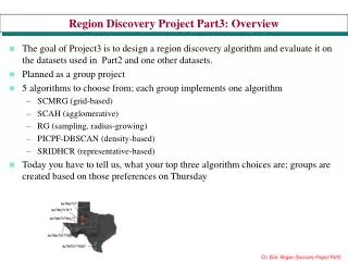
1. Region Discovery Project Part3: Overview • The goal of Project3 is to design a region discovery algorithm and evaluate it on the datasets used in Part2 and one other datasets. • Planned as a group project • 5 algorithms to choose from; each group implements one algorithm • SCMRG (grid-based) • SCAH (agglomerative) • RG (sampling, radius-growing) • PICPF-DBSCAN (density-based) • SRIDHCR (representative-based) • Today you have to tell us, what your top three algorithm choices are; groups are created based on those preferences on Thursday

2. Region Discovery Part3: Clustering Algorithms • The objective of Part3 is to design and implement a clustering/region discovery algorithm that returns a set of regions that maximize a given fitness function q for a given spatial dataset. Inputs of the designed algorithm include: • Clustering algorithm specific parameters (e.g. grid-cell size, number of clusters c) • Parameter b of q(X) • Measure of Interestingness i(r) used including measure specific parameters (e.g. shape parameter  in some fitness functions) • The region discovery algorithm to be designed returns the set of clusters (regions) and their associated interestingness and cluster reward; each cluster is described by triples (<set of objects belonging to the cluster>, <interestingness>, <cluster_reward>).

3. Region Discovery Part3: Preview Representative-based Algorithms • Using PAM with fitness function q for a fixed numbers of k regions. Functions when implementing this algorithm include: • Implementation of an initialization function that selects k-representatives at random. • Creating clusters for a given set of representatives • Creating new sets of representatives by replacing a representative by a single non-representative • SRIDHCR (see next transparencies) is a representative-based clustering that, in contrast to PAM, removes representatives and adds new representatives to the current set of representatives (see next set of transparencies)

4. Version of the PAM Algorithm for Region Discovery • Randomly create an initial set of k representatives curr • WHILE NOT DONE DO • Create new solutions S by replacing a single representative in curr by a single non-representative. • Determine the element s in S for which q(s) is maximal (if there is more than one minimal element, randomly pick one). • IF q(s)>q(curr) THEN curr:=s • ELSE terminate, returning curr as the solution for this run. curr: current set of cluster representatives Not an algorithm to choose from in the course project!

5. REPEAT r TIMES • curr := a randomly created set of representatives (with size between k’ and 2*k’) • WHILE NOT DONE DO • Create new solutions S by adding a single non-representative to curr and by removing a single representative from curr. • Determine the element s in S for which q(s) is the largest (if there is more than one maximal element, randomly pick one). • IF q(s)>q(curr) THEN curr:=s • ELSE IF q(s)=q(curr) AND |s|<|curr| THEN curr:=s • ELSE terminate and return curr as the solution for this run. • Report the best out of the r solutions found. Algorithm SRIDHCR Remark: c, and r, and k’ are input parameters.

6. Example SRIDHCR. In this example, we assume q(X) has to be minimized

7. SCAH (Agglomerative Hierarchical) Inputs: A dataset O={o1,...,on} A distance Matrix D = {d(oi,oj) | oi,oj O }, Output: Clustering X={c1,…,ck} Algorithm: 1) Initialize: Create single object clusters: ci = {oi}, 1≤ i ≤ n; Compute merge candidates based on “nearest clusters” MERGE-CANDIDATE(c1,c2)= if c1 is closest to c2 or c2 is closest to c1 2) DO FOREVER a) Find the pair (ci, cj) of merge candidates that improves q(X) the most b) If no such pair exist terminate, returning X={c1,…,ck} c) Delete the two clusters ci and cjfrom X and add the cluster ci  cj to X d) Update inter-cluster distances incrementally e) Update merge candidates based on inter-cluster distances Recommendation: Use min-dist/single link to compute inter-cluster distances

8. Ideas SCMRG (Divisive, Multi-Resolution Grids) Cell Processing Strategy 1. If a cell receives a reward that is larger than the sum of its rewards its ancestors: return that cell. 2. If a cell and its ancestor do not receive any reward: prune 3. Otherwise, process the children of the cell (drill down)

9. ‘SCMRG Simple’ Pseudo Code • Put initial cells with flag set to false on the queue • WHILE queue NOT EMPTY DO • c=pop(queue) • If a cell c receives a reward that is larger than the sum of its rewards its ancestors: add c to the results reported • If a cell c has stop=false and its ancestors do not receive any reward: put its ancestors on the queue with stop=true • If a cell c has stop=true and its ancestors do not receive any reward: prune that cell. • Otherwise, process the children q of the cell (drill down) by putting (false,q) on the queue Remark: cells have a Boolean flag called stop for pruning; the queue contains (<stop-flag>,<cell>) Idea: Use queue of work still to be done as the main data structure.

10. Code SCMRG

11. PICPF-DBSCAN Input parameters: plug-in core-point function corep, radius r • For each point p in the dataset, compute the region r=(p,r) and determine if it is a core-point by calling corep(p,r) • Create clusters as DBSCAN does Examples of Plug-in Core-point Functions: • The region r contains 3 other points and its purity is above 80% • The regions r contains 5 other points and the standard deviation of the continuous variable is at least twice as much as the standard deviation for the whole dataset. • The region r contains 4 other points—simulates DBSCAN Minpts=4 Remarks: • It is okay to modify an existing implementation of DBSCAN if you find one… • Does not fit 100% into the region discovery framework; therefore, experiments have to be slightly modified.

12. Region Growing Algorithm (RG)Algorithm Sketch Input parameters: r (size of radius), y (how many points will be selected to draw radii around) • Create a result data-structure Top10 that contains the top ten regions found so far sorted by their q(X) value. • DO y TIMES • Randomly select a point p=(<x>,<y>) (does not need to be a point in the dataset) • Draw radiuses of size r, 1.1*r, 1.3*r, 1.7*r, 2.2*r, 2.8*r, 3,5*r, 4.3*r, 5,2*r, 6.3*r around p “in general, follow some schedule to increase r” • Add the region, computed in step 2, with the higher q(X) value to TOP10 • Return the top ten regions and the sum of their rewards Remarks: • Returns overlapping regions • Only returns the top 10 regions • Similar to the popular SATSCAN hotspot discovery algorithm • Can be generalized by making k (10 in the above) to be an input parameter X

13. Not that important this year!!! Region Discovery Project Part3: Visualization Issues • Data sets (without regions, prior to region discovery) • Visualize spatial objects in the dataset • Visualize class labels for supervised data sets in different colors • If datasets have a continuous variables, discretize them and display them like supervised datasets using an ordinal color coding(e.g. blue  yellow) • Data sets with regions (final or intermediate result of a region discovery alg.) • Region boundaries (draw a border around a region) • If a representative-based clustering algorithm was used, display the region representative for each region • Objects that belong to a region • Interestingness and reward of a region • Other region characteristics (vary for different measures of interestingness and for different region discovery tasks) • Display an individual region (e.g. the one that received the highest reward) • Use similar techniques as in 2. • Ideally, maps should be used as the background of displays to provide reference information and to make the display look nicer.

14. Example: Discovery of “Interesting Regions” in Wyoming Census 2000 Datasets Ch. Eick

15. Problems with SCAH Too restrictive definition of merge candidates: XXXOOO OOOXXX No look ahead: Non-contiguous clusters:

16. More on Grid Structures • Grid-cells are pairs of integers (i,,j) with i and j being numbers between 0 and g-1 • Let v be a value of the attribute att, then the number of v’s grid-cell is computed as follows: g’= floor ((v - att_min)*g)/(att_max - att_min)) Example: Let attribute att1 range between -50 and +50 and att2 range between 0 and 20 and g is 10, and an example e=(att1=-5,att2=17) is given. Example e is assigned to the grid-cell (4,8), because floor=(-5 – (-50))x10)/100)= floor(450/100)=4 and floor(((17-0)x10)/20)=floor(8.5)=8 • For a 2D grid-structure the following holds: • two different cells (i1,j1) and (i2,j2) are merge-candidates  i1=i2 or j1=j2