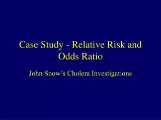
Case Study - Relative Risk and Odds Ratio
110 likes | 454 Views
Case Study - Relative Risk and Odds Ratio. John Snow’s Cholera Investigations. Population Information. 2 Water Providers: Southwark & Vauxhall (S&V) and Lambeth (L) S&V: Population: 267625 # Cholera Deaths: 3706 L: Poulation: 171528 # Choleta Deaths: 411.

Case Study - Relative Risk and Odds Ratio
E N D
Presentation Transcript
Case Study - Relative Risk and Odds Ratio John Snow’s Cholera Investigations
Population Information • 2 Water Providers: Southwark & Vauxhall (S&V) and Lambeth (L) • S&V: Population: 267625 # Cholera Deaths: 3706 • L: Poulation: 171528 # Choleta Deaths: 411
Sampling Distribution of RR & OR • Goal: Obtain Empirical Sampling Distributions of sample RR and OR and observe coverage rate of 95% Confidence Intervals • Process: Take independent random samples of size nSV and nL from the 2 populations and observe XSV and XL deaths in sample. These XSV and XL are approximately distributed as Binomial random variables (approximate due to sampling from finite, but very large, populations)
Binomial Distribution for Sample Counts • Binomial “Experiment” • Consists of n trials or observations • Trials/observations are independent of one another • Each trial/observation can end in one of two possible outcomes often labelled “Success” and “Failure” • The probability of success, p, is constant across trials/observations • Random variable, X, is the number of successes observed in the n trials/observations. • Binomial Distributions: Family of distributions for X, indexed by Success probability (p) and number of trials/observations (n). Notation: X~B(n,p)
Binomial Distributions and Sampling • Problem when sampling from a finite sample: the sequence of probabilities of Success is altered after observing earlier individuals. • When the population is much larger than the sample (say at least 20 times as large), the effect is minimal and we say X is approximately binomial • Obtaining probabilities: Table C gives probabilities for various n and p. Note that for p > 0.5, use 1-p and you are obtaining P(X=n-k)
Simulating Binomial RVs • Select n and p • Obtain n random numbers distributed uniformly between 0 and 1 (any software package should have built-in random number generator): U1,…,Un • Let X be the number of Uivalues that p • X~B(n,p) • Finite population adjustments can be made by “correcting” p after each draw • EXCEL has built in Function: • Tools --> Data Analysis --> Random Number Generation • --> Binomial --> Fill in p and n
Simulation Example • Simulate by taking samples of nSV=nL=5000 individuals from each population of customers • Generate XSV~B(5000,.013848) and XL~B(5000,.002396) • Compute sample relative risk, ln(RR), odds ratio, ln(OR), and estimated std. errors of ln(RR) and ln(OR) • Obtain 95% CIs for RR, OR (based on ln(RR),ln(OR) • Repeat for a large number of samples (1000 samples) • Obtain the empirical distribution of each statistic • Obtain an indicator of whether the 95% CI for RR contains the population RR (5.78) and whether the 95% CI for OR contains the population OR (5.85)