Parallel OpenCL-based Solver for Large-Scale DNS of Incompressible Flows
270 likes | 297 Views
This paper presents a parallel OpenCL-based solver for performing large-scale Direct Numerical Simulations (DNS) of incompressible flows. The solver is capable of simulating incompressible turbulent flows with heat transfer using high-order numerical schemes. It has high spatial and temporal resolution and can handle complex physical phenomena in simplified geometries. The solver has been validated for various test cases including differentially heated cavity, surface-mounted cube, impinging jet, square cylinder, and square duct. The algorithm of the solver consists of a Navier-Stokes system, an energy equation, and a Poisson equation solver. It has been parallelized using MPI+OpenMP two-level parallelization and can be further extended to utilize GPUs with OpenCL.

Parallel OpenCL-based Solver for Large-Scale DNS of Incompressible Flows
E N D
Presentation Transcript
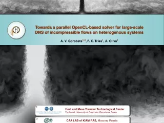
Towards a parallel OpenCL-based solver for large-scale DNS of incompressible flows on heterogenous systems A. V. Gorobets1,2, F. X. Trias1, A. Oliva1 1 Heat and Mass Transfer Technological Center Technical University of Catalonia, Barcelona, Spain 2 CAA LAB of KIAM RAS, Moscow, Russia
Applications with high computing power demands Direct numerical simulations of incompressible flows ●Incompressible turbulent flows with heat transfer ●High order numerical schemes ●Simplified geometry but complex physical phenomena ●High space and time resolution, long time integration period ●Validation basis for turbulence models Differentially heated cavity Ra up to 1012 (110M nodes) Surface mounted cube, Re=7300 (16M nodes) Impinging jet, Re=20000 (100M nodes) Square cylinder, Re=22K (75M nodes) Square duct, Re_tau=1200 (170M nodes)
A CFD algorithm for incompressible flows ●Navier-Stokes system to solve: . The algorithm of the time step ●Discrete system for pressure-velocity coupling: • Predictor velocity field, , is obtained explicitly • Correction, , is obtained from thePoissonequation • Resulting velocity field, , is obtained • Energy equation is solved explicitly where ●Fractional step projection method: Predictor velocity: where Unknown velocity: Mass conservation equation: The Poisson equation
The Poisson solver for cases with one periodic direction ●The method is based on a time-consuming preprocessing ●Allows flexible configuration for different parallel systems, CPU groups and problem sizes ●3D geometry is restricted to extruded 2D shapes with a constant mesh step, so called “2.5D” ●A multigrid-like extension makes the solver applicable for fully 3D configurations The algorithm of the solver • Fourier diagonalization using FFT uncouples 3D problem into set of independent 2D problems (planes) • The Schur complement based direct method is used to solve planes that correspond to lower Fourier frequencies • The preconditioned conjugate gradient (PCG) method is used to solve the remaining planes • Inverse FFT to restores solution of the 3D problem. Uncoupling of a 3D domain using FFT Gorobets, F. X. Trias, M. Soria and A. Oliva, “A scalable parallel Poisson solver for three-dimensional problems with one periodic direction”, Computers & Fluids journal, 39 (2010) 525-538, Elsevier
The MPI+OpenMP two-level parallelization MPI parallelization ●Domain is decomposed into P = Px x Pyz parts in all 3 directions ●Periodic direction is decomposed in Px parts: FFT is replicated within 1D groups and each FFT is sequential. ●Each plane is decomposed into Pyz parts ●First D planes are solved with the direct method, the remaining planes with the iterative method OpenMP parallelization ●Explicit part is parallelized by decomposing loops over nodes ●FFT stages (1,4) are parallelized in the same way: set of subvectors is divided between threads FFT itself stays sequential! ●The set of planes is divided between threads on stages 2, 3 ●I/O and MPI communications are performed by thread 0 A. Gorobets, F. X. Trias, R. Borrell, O. Lehmkuhl, A. Oliva, “Hybrid MPI+OpenMP parallelization of an FFT-based 3D Poisson solver with one periodicdirection”, Elsevier, Computers & Fluids (2011)
Speedups with MPI+OpenMP Speedup varying Pt, Pyz=64, Px=1, MVS100K ●In total P = Px x Pyzx Pt CPU cores engaged ●With Px=8 and Pt=8 the solver reaches its limits on 8-core nodes ●However Pyz = 200 is still far from its limits, 12800 cores just was maximum available for tests ●Till Pyz = 800 it works well, so we estimate limits as at least 800x8x8 =51200CPU cores ●Symmetric extension for cases with domain symmetry allows to scale this number up to 4 times leading beyond 105cores Speedups varying Px, Pyz=200, Pt=8, Lomonosov supercomputer Speedup varying Pyz, Pt=8, Px=1, Lomonosov Mesh2: 330 millions of nodes Mesh3: 1003 millions of nodes
Extension of the parallel model “usual” supercomputer supercomputer with hybrid nodes ●Nodes of a supercomputer are coupled by means of MPI within distributed memory model and MIMD parallelism ●OpenMP provides parallelization inside multi-core nodes within shared memory model and the same MIMD parallelism ●OpenCL engagesGPUs, where SIMD is used on the level of SMs
Using GPUs A program for a heterogeneous system consists of a CPU code, so called host code, and a GPU code, so called kernel code. ●CUDA - Compute Unified Device Architecture Is now most popular, can work only on NVidia hardware ●OpenCL - Open Computing Language works on both NVidia and AMD (ATI) OpenCLwas chosen for its portability Comparison of GPUvs. CPU ●Streaming processors with SIMDparallelism ●Much more cores – hundreds, thousands ●Latency hiding for memory access ●Complex memory hierarchy ●5-6 times bigger memory bandwidth ●2-3 times more power consumption ●>3 times more expensive (NVidia) OpenCL memory model NVIdia Fermi
Interconnection 5.6Gbit Latency 10-6 sec. PCI-Express Node Node Node Node Node Node Node Node Computing node 12 CPU cores at 2.93 GHz 96 Gb RAM DDR3 3 GPU NVidia C2050: 3x448=1344 cores 3x2.5 = 7.5 Gb DDR5 Supercomputer К100 (www.kiam.ru) Equipment Reference CPU: ●Intel Xeon X5670 2.93GHz 12Gflops, 32Gb/s GPU devices: ●NVidia Tesla C2050 (K100)●AMD Radeon 7970 ●NVidia GeForce GTX480●AMD Radeon 6970 515Gflops, 144Gb/s 947 Gflops, 264Gb/s 164Gflops, 177Gb/s 683Gflops, 176Gb/s Computing module NIISI RAS
The overall algorithm and basic operations • ●Momentum equation • diffusion operator (3 x op. 1) • convection operator (3 x op. 2) • mass force term (op. 1) • summation of terms (3 x op. 3.3) • ●Energy eq. • diffusion operator (op. 1) • convection operator (op. 2) • summation of terms (op. 3.3) • ●Intermediate calculations • get predictor fields (some linear field operation) • boundary conditions for velocity and temperature • calculate divergence field, the r.h.s. for the Poisson eq. (op. 1 x 3) • ●Mass conservation eq. - Poisson • FFT (op. 4) • DSD for planes 1,..,D - on CPU • CG for planes D,..,Nx • SpMV (op. 5), dot product • IFFT (op. 4) • ●Intermediate calculaitons • gradient calculation (op.1 x 3) • linear field operations to get resulting velocity field • ●Time integration step, average fields processing • linear field operations • ●Halo update Basic operations 1.Diffusion stencil product 2.Convection stencil product 3.Linear field operations: y = a1*x1+…+an*xn + c; n from 1 to 4 4.FFT and IFFT 5.Sparse matrix vector product c o m p l e t e communications GPU → CPU: D planes of r.h.s. vector GPU → CPU→ GPU: halos, dots CPU → GPU: D planes of solution vector t o d o GPU → CPU→ GPU: halos
Extended subdomain border Subdomain nodes Borders between subdomains Halo nodes stencil subdomain halo Details on stencil product computing pattern Diffusion stencil product ●It is in fact a 19-diagonal SpMV u = Dv for “3D” vectors of size N = Nxx Nyz ●The matrix consists of Nx equal blocks hence only one “2D”block of size Nyz is stored ●The stencil is stored as 19 fields flattened in 1D vectors ●Offsets in all directions are pre-calculated for fast access to neighboring nodes for the center node (i,j,k) positioned in memory at P-th array position (i+1,j,k) is at P+1, (i,j+1,k) is at P+off_y, (i,j,k) at P+off_z instead of calculating position directly by #define _AMD_3D(i,j,k) ((i-OFFX) + (j-OFFY)*Nx + (k-OFFZ)*Nxy) where OFFX, OFFY, OFFZ – halo offsets ●Preprocessor macro programming is extensively used Diffusion stencil
Details on stencil product computing pattern // array field access macro: #define _AMD_2D(i,j) ((i-OFFY) + (j-OFFZ)*TY) #define _AMD_3D(i,j,k) ((i-OFFX) + (j-OFFY)*TX + (k-OFFZ)*TXTY) // stencil coefficients and advection field product macro: #define MULSTENCIL(aa) \ { \ for(int s=0; s<st_ssize##aa; s++){ /*loop over stencil nodes */ \ const double buf1=bufStencil[p2d]; bufStencil+=sfsize; /* left coef */ \ const double buf2=bufStencil[p2d]; bufStencil+=sfsize; /* right coef*/ \ const int offst3Daa = offst3D##aa*(s+1); /*offset between neighboring levels*/ \ pr += buf1*sfphi[p3d0-offst3Daa] + buf2*sfphi[p3d0+offst3Daa]; \ } \ } __kernel void STENCIL_GPU(__global double *sfphi, __global double *prphi, __global double *bufStencil){ const int I = get_global_id(0)/ls; const int lID = get_global_id(0)%ls; int p2d, p3d0; { const int i1 = I%NY+offY, i2 = I/NY+offZ; p2d = _AMD_2D(i1,i2); p3d0 = _AMD_3D(offX+lID,i1,i2); } /*central node*/ double pr = bufStencil[p2d]*(sfphi[p3d0]); bufStencil+=sfsize; MULSTENCIL(0); MULSTENCIL(1); MULSTENCIL(2); prphi[p3d0]=pr; } #define TX 70 #define TY 92 #define TXTY 6440 #define NX 60 #define NY 80 #define NZ 160 #define NYZ 12800 #define OFFX 1 #define OFFY -4 #define OFFZ -4 #define offX 6 #define offY 2 #define offZ 2 #define add 0 #define sfsize 0 #define ls 1 #define ssizemax 0 #define offst3D0 1 #define offst3D1 70 #define offst3D2 6440 #define st_ssize0 0 #define st_ssize1 0 #define st_ssize2 0 #define st_pos0 0 #define st_pos1 0 #define st_pos2 0
Details on stencil product computing pattern • Convection stencil product • ●Is much more complicated, since C is C(v), where v is the current velocity field, and since the mesh is • staggered calculation of indexes turns to a mess • ●To compute each resulting coefficient of the stencil a variable number of pre-calculated values is needed • its number is less or equal to the size of the stencil legs. • ●The data structure that represents a stencil is following: • int *st_nr// numbers of “pre-coefficient” positions for each node • int *st_spos// stencil data position for each node • int *st_i, // indexes of neighbours for each stencil node • double *st_coef // stencil coefficients • ●Computing each stencil coefficient looks like this: • // stencil coefficients and advection field product macro: • #if(ssizemax==1) /*lo order scheme*/ • #define GET_BCPV(padv) \ • (((nr>0) ? bcoef[0]*padv[bi[0]] : 0.0) + \ • ((nr>1) ? bcoef[1]*padv[bi[1]] : 0.0)) • #else /*high order*/ • #define GET_BCPV(padv) \ • (((nr>0) ? bcoef[0]*padv[bi[0]] : 0.0) + \ • ((nr>1) ? bcoef[1]*padv[bi[1]] : 0.0) + \ • ((nr>2) ? bcoef[2]*padv[bi[2]] : 0.0) + \ • ((nr>3) ? bcoef[3]*padv[bi[3]] : 0.0)) • #endif b2t2 b3t2 b1t2 b4t2
Poisson solver GPUzation ●DSD solver is fully on CPU – too much MPI traffic and complexity ●CG – approx. inverse or two-level preconditioned with block-CG ●Multi-SpMV, multi-dot – communications combined for all remaining planes ●Communication and computation overlap for MPI and GPU-CPU comms The algorithm of the solver • Fourier diagonalization using FFT uncouples 3D • problem into set of independent 2D problems (planes) • The Schur complement based direct method is used to solve planes that correspond to lower Fourier frequencies • The preconditioned conjugate gradient (PCG) method is used to solve the remaining planes • Inverse FFT to restores solution of the 3D problem. • Operations of the solver • FFT (op. 4) • DSD for planes 1,..,D - on CPU • CG for planes D,..,Nx • SpMV (op. 5), dot product • IFFT (op. 4) communications GPU → CPU: D planes of r.h.s. vector GPU → CPU→ GPU: halos, dots CPU → GPU: D planes of solution vector
Performance on GPU Net performance, Gflops* The test case ●DHC typical case is used ● 4-th order scheme ●Mesh sizes 430K, 770K,1.2M nodes ●Imitates a typical computing load % of peak *by fairly counting the number of operations in the algorithms 1 CPU core vs 1 GPU 6-cored Xeon vs 1 GPU* *assuming typical OpenMP speedup 4.5 out of 6 cores
Overal multi-GPU parallel model ●CPUs only for control, MPI comms and DSD – if GPU is much faster MPI – 1st level 2nd level domain decomposition OpenCL – 3rd level ●CPUs and GPUs are computing together - if CPU is comparable to GPU MPI – 1st level 2nd level domain decomposition OpenMP – 3rd level OpenCL – 3rd level
Technology of porting operations ● Each operation has standalone separated test that loads all the input data from file ●Each operation has GPUzed CPU version ●Everything scalar known at the time of kernel compilation taken to defined constants ●Loops unrolled, branching replaced with preprocessor commands ●Positioning pre-calculated and added as defined constants ●Divisions minimized ●Data access reorganized for achieving coalescing ●Data is properly aligned ●Usage of registers is minimized ●Workgroup size optimized for particular device ●Additional correctness control is implemented for each operation
General conclusions • ● AMD is much faster than NVidia • ●On CPU-like kernels NVidia 2050 is ~5-10 times slower than AMD 7970 • (record so far is 12) • ●On kernels optimized for NVidia its 2050 is ~2-3 times slower than AMD 7970 • ●AMD software is shameful! • ●CUDA easier than OpenCL – is a dramatic delusion • ●OpenCL portability is illusion: it works on everything but may work very slow until optimized for • particular architecture • ●CUDA faster than OpenCL – very questionable statement • in most cases performance is equal, however we observed 10-15% slowdown on certain kernels • ●What works well on NVidia works well on AMD. • What works well on AMD may appear 10 times slower on NVidia. • ●Optimization priority should be NVidia architecture since its more weak • ●OpenCL works well on CPU. OpenCL vs. OpenMP showed like 4.3 vs. 4.5 speedup on 6-cored Xeon NVidia → AMD: yes AMD → NVidia: no
Flops vs Gb/s ● 7970 has 950 Gflops and 264 Gb/s hence we need 3.6 flop per byte to get those flops ● 2050 has 515 Gflops and 144 Gb/s, so the same 3.6 flop per byte to get those flops ● This means around 30 flop per one double! ● Our stencil product say roughly around 0.25 flops per byte or 2 flop per double… ●GTX480 with its pitiful 164 Gflops outperformed 2050 around 30%. Memory bandwidth is far more important than flops
CUDA vs OpenCL CUDA ●Much better infrastructure – manuals, tutorials, support ●In rare cases little better performance ●More software and libs available ●Compilation together with CPU code ●Vendor-locked ●Oriented on particular architecture OpenCL ●More advanced and elegant programming model ●Compilation during runtime of CPU code ●Supported by major hardware vendors – NVidia, AMD, Intel, Apple, … ●Fits wide range of architectures – CPU, GPU, … ●No to Fortran
AMD vs nVidia nVidia ●Much better infrastructure ●Better software ●Brutally overpriced GPGPUs – x10 price for the same chip ●More weak architecture, poor and sometimes very poor performance AMD ●Eats not adapted CPU code much better, hence easier to program ●Bigger memory bandwidth and computing power ●Times faster. Order of magnitude sometimes. Due to advantage in architecture as well ●Software is a shame! Needs window session to be opened, hangs, fails. A mixture of AMD GPU chip and nVidia soft would lead to an ideal
CPU vs GPU Power consumption ● ~100 Wt for 6 core Xeon ● ~250 Wt for GPU Speedup must be >2.5 vs Xeon or > 12 vs 1 core Price ● ~1K for Xeon ● ~3K for Tesla Speedup must be >3 vs Xeon or > 13.5 vs 1 core Complexity, effort, .. ? ..but if the system is available who cares about speedup? CPU+GPU must just be faster than CPU
Conclusions Our recent DNS of a square duct at Re_tau=1200, 170M nodes ● GPU is not for kids ●Things rapidly changing and future is not clear ●The large-scale multi-level parallel CFD solver for hybrid systems to be finished soon! Thanks for your attention!
Symmetric extension Symmetric extension for cases with mesh symmetries ●The original system to solve: ●Changing basis in the following way: The vector is decomposed into symmetric and skew-symmetric parts: ●Applying change of basis to the linear system: The algorithm is following: • Transform the right-hand-side sub-vector, • Solve the two decoupled systems, • Reconstruct solution, ●Stages 1 and 3 require a point-to-point communication
CPU vs GPU Total 1 37.945032 37.945032 100.00 cr_info: GPU write 10 0.018545 0.185451 0.49 cr_info: r_cdm 10 0.385833 3.858332 10.17 cr_info: rc_cdm 10 0.250128 2.501276 6.59 cr_info: prod_nl_stencil_scaf 30 0.083371 2.501128 6.59 cr_info: rd_cdm 10 0.080982 0.809824 2.13 cr_info: prod_stencil_scaf 40 0.026940 1.077591 2.84 cr_info: rf_cdm 10 0.026800 0.267998 0.71 cr_info: op: cl_3vecf 10 0.027911 0.279112 0.74 cr_info: r_cdm_GPUzed 10 0.021045 0.210450 0.55 cr_info: rc_cdm_GPU 10 0.014247 0.142465 0.38 cr_info: NL_STENCIL_GPU 10 0.014245 0.142453 0.38 cr_info: rd_cdm_GPU 10 0.003601 0.036014 0.09 cr_info: D STENCIL_GPU 10 0.003600 0.036001 0.09 cr_info: rf_cdm_GPU 10 0.001275 0.012755 0.03 cr_info: F STENCIL_GPU 10 0.001274 0.012741 0.03 cr_info: op: cl_3vecf_GPUzed 10 0.001917 0.019167 0.05 cr_info: GPU read 1 0.050634 0.050634 0.13 cr_info: Total 1 24.007549 24.007549 100.00 cr_info: GPU write 10 0.038326 0.383260 1.60 cr_info: r_cdm 10 0.371780 3.717800 15.49 cr_info: rc_cdm 10 0.233489 2.334894 9.73 cr_info: prod_nl_stencil_scaf 30 0.077825 2.334750 9.73 cr_info: rd_cdm 10 0.082973 0.829735 3.46 cr_info: prod_stencil_scaf 40 0.027621 1.104841 4.60 cr_info: rf_cdm 10 0.027535 0.275351 1.15 cr_info: op: cl_3vecf 10 0.027771 0.277709 1.16 cr_info: r_cdm_GPUzed 10 0.009513 0.095134 0.40 cr_info: rc_cdm_GPU 10 0.006281 0.062814 0.26 cr_info: NL_STENCIL_GPU 10 0.006280 0.062797 0.26 cr_info: rd_cdm_GPU 10 0.001634 0.016338 0.07 cr_info: D STENCIL_GPU 10 0.001632 0.016320 0.07 cr_info: rf_cdm_GPU 10 0.000616 0.006161 0.03 cr_info: F STENCIL_GPU 10 0.000614 0.006140 0.03 cr_info: op: cl_3vecf_GPUzed 10 0.000976 0.009764 0.04 cr_info: GPU read 1 0.099515 0.099515 0.41 ================================================== Convection: 0.490571 sec, 43.9387 GFlops, 17.189 Gb/s ================================================== ================================================== Diffuion: 0.132634, 75.2388 GFlops ================================================== cr_info: Total 1 25.387849 25.387849 100.00 cr_info: GPU write 10 0.014997 0.149967 0.59 cr_info: r_cdm 10 0.241860 2.418604 9.53 cr_info: rc_cdm 10 0.159842 1.598423 6.30 cr_info: prod_nl_stencil_scaf 30 0.053276 1.598270 6.30 cr_info: rd_cdm 10 0.047335 0.473349 1.86 cr_info: prod_stencil_scaf 40 0.015823 0.632934 2.49 cr_info: rf_cdm 10 0.015979 0.159794 0.63 cr_info: op: cl_3vecf 10 0.018693 0.186928 0.74 cr_info: r_cdm_GPUzed 10 0.013812 0.138117 0.54 cr_info: rc_cdm_GPU 10 0.009267 0.092669 0.37 cr_info: NL_STENCIL_GPU 10 0.009266 0.092657 0.36 cr_info: rd_cdm_GPU 10 0.002371 0.023713 0.09 cr_info: D STENCIL_GPU 10 0.002369 0.023691 0.09 cr_info: rf_cdm_GPU 10 0.000870 0.008705 0.03 cr_info: F STENCIL_GPU 10 0.000869 0.008685 0.03 cr_info: op: cl_3vecf_GPUzed 10 0.001298 0.012977 0.05 cr_info: GPU read 1 0.038492 0.038492 0.15
Performance on GPU ================================================== Convection: 0.231484 sec, 93.1169 Flops, 36.4277 Gb/s ================================================== ================================================== Diffuion: 0.068738 150 ================================================== cr_info: nom o N mode tsum tavg (s) percentage cr_info: Total 1 15.700642 15.700642 100.00 cr_info: GPU write 10 0.025440 0.254405 1.62 cr_info: r_cdm 10 0.231576 2.315758 14.75 cr_info: rc_cdm 10 0.147438 1.474383 9.39 cr_info: prod_nl_stencil_scaf 30 0.049142 1.474256 9.39 cr_info: rd_cdm 10 0.049354 0.493539 3.14 cr_info: prod_stencil_scaf 40 0.016448 0.657906 4.19 cr_info: rf_cdm 10 0.016456 0.164559 1.05 cr_info: op: cl_3vecf 10 0.018319 0.183186 1.17 cr_info: r_cdm_GPUzed 10 0.006380 0.063796 0.41 cr_info: rc_cdm_GPU 10 0.004099 0.040988 0.26 cr_info: NL_STENCIL_GPU 10 0.004097 0.040972 0.26 cr_info: rd_cdm_GPU 10 0.001122 0.011223 0.07 cr_info: D STENCIL_GPU 10 0.001120 0.011202 0.07 cr_info: rf_cdm_GPU 10 0.000444 0.004441 0.03 cr_info: F STENCIL_GPU 10 0.000442 0.004424 0.03 cr_info: op: cl_3vecf_GPUzed 10 0.000708 0.007084 0.05 cr_info: GPU read 1 0.067318 0.067318 0.43 cr_info: Total 1 25.387849 25.387849 100.00 cr_info: GPU write 10 0.014997 0.149967 0.59 cr_info: r_cdm 10 0.241860 2.418604 9.53 cr_info: rc_cdm 10 0.159842 1.598423 6.30 cr_info: prod_nl_stencil_scaf 30 0.053276 1.598270 6.30 cr_info: rd_cdm 10 0.047335 0.473349 1.86 cr_info: prod_stencil_scaf 40 0.015823 0.632934 2.49 cr_info: rf_cdm 10 0.015979 0.159794 0.63 cr_info: op: cl_3vecf 10 0.018693 0.186928 0.74 cr_info: r_cdm_GPUzed 10 0.013812 0.138117 0.54 cr_info: rc_cdm_GPU 10 0.009267 0.092669 0.37 cr_info: NL_STENCIL_GPU 10 0.009266 0.092657 0.36 cr_info: rd_cdm_GPU 10 0.002371 0.023713 0.09 cr_info: D STENCIL_GPU 10 0.002369 0.023691 0.09 cr_info: rf_cdm_GPU 10 0.000870 0.008705 0.03 cr_info: F STENCIL_GPU 10 0.000869 0.008685 0.03 cr_info: op: cl_3vecf_GPUzed 10 0.001298 0.012977 0.05 cr_info: GPU read 1 0.038492 0.038492 0.15