Last Two Lectures
660 likes | 843 Views
Last Two Lectures. Panoramic Image Stitching. Feature Detection and Matching. Today. More on Mosaic. Projective Geometry. Single View Modeling. Vermeer’s Music Lesson. Reconstructions by Criminisi et al. Image Alignment. Feature Detection and Matching. Cylinder: Translation 2 DoF.

Last Two Lectures
E N D
Presentation Transcript
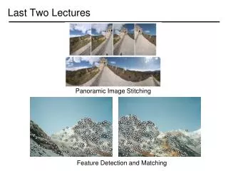
Last Two Lectures Panoramic Image Stitching Feature Detection and Matching
Today More on Mosaic Projective Geometry Single View Modeling Vermeer’s Music Lesson Reconstructions by Criminisi et al.
Image Alignment Feature Detection and Matching Cylinder: Translation 2 DoF Plane: Homography 8 DoF
Plane perspective mosaics • 8-parameter generalization of affine motion • works for pure rotation or planar surfaces • Limitations: • local minima • slow convergence
(Xc,Yc,Zc) xc f x Revisit Homography
Absolute orientation [Arun et al., PAMI 1987] [Horn et al., JOSA A 1988]Procrustes Algorithm [Golub & VanLoan] • Given two sets of matching points, compute R such that pi’ = R pi • A = Σipipi’T = U S VT • R = VUT
(Xc,Yc,Zc) xc f x What if we don’t know f? { H
The drifting problem • Error accumulation • small errors accumulate over time
Bundle Adjustment Associate each image i with Each image i has features Trying to minimize total matching residuals
Rotations • How do we represent rotation matrices? • Axis / angle (n,θ)R = I + sinθ [n] + (1- cosθ) [n]2(Rodriguez Formula), with [n] be the cross product matrix.
Incremental rotation update • Small angle approximationΔR = I + sinθ [n] + (1- cosθ) [n]2 ≈ I +θ [n] = I+[ω]linear inω= θn • Update original R matrixR ← RΔR
Recognizing Panoramas [Brown & Lowe, ICCV’03]
Get you own copy! [Brown & Lowe, ICCV 2003] [Brown, Szeliski, Winder, CVPR’05]
How well does this work? Test on 100s of examples…
How well does this work? Test on 100s of examples… …still too many failures (5-10%)for consumer application
Matching Mistakes: False Negative • Moving objects: large areas of disagreement
Matching Mistakes • Accidental alignment • repeated / similar regions • Failed alignments • moving objects / parallax • low overlap • “feature-less” regions(more variety?) • No 100% reliable algorithm?
How can we fix these? • Tune the feature detector • Tune the feature matcher (cost metric) • Tune the RANSAC stage (motion model) • Tune the verification stage • Use “higher-level” knowledge • e.g., typical camera motions • → Sounds like a big “learning” problem • Need a large training/test data set (panoramas)
on to 3D… Enough of images! We want more from the image We want real 3D scene walk-throughs: Camera rotation Camera translation
So, what can we do here? • Model the scene as a set of planes!
(x,y,1) image plane The projective plane • Why do we need homogeneous coordinates? • represent points at infinity, homographies, perspective projection, multi-view relationships • What is the geometric intuition? • a point in the image is a ray in projective space y (sx,sy,s) (0,0,0) x z • Each point(x,y) on the plane is represented by a ray(sx,sy,s) • all points on the ray are equivalent: (x, y, 1) (sx, sy, s)
A line is a plane of rays through origin • all rays (x,y,z) satisfying: ax + by + cz = 0 l p • A line is also represented as a homogeneous 3-vector l Projective lines • What does a line in the image correspond to in projective space?
l1 p l l2 Point and line duality • A line l is a homogeneous 3-vector • It is to every point (ray) p on the line: lp=0 p2 p1 • What is the line l spanned by rays p1 and p2 ? • l is to p1 and p2 l = p1p2 • l is the plane normal • What is the intersection of two lines l1 and l2 ? • p is to l1 and l2 p = l1l2 • Points and lines are dual in projective space • given any formula, can switch the meanings of points and lines to get another formula
(a,b,0) y y (sx,sy,0) z z image plane image plane x x • Ideal line • l (a, b, 0) – parallel to image plane Ideal points and lines • Ideal point (“point at infinity”) • p (x, y, 0) – parallel to image plane • It has infinite image coordinates • Corresponds to a line in the image (finite coordinates)
Homographies of points and lines • Computed by 3x3 matrix multiplication • To transform a point: p’ = Hp • To transform a line: lp=0 l’p’=0 • 0 = lp = lH-1Hp = lH-1p’ l’ = lH-1 • lines are transformed bypostmultiplication of H-1
3D projective geometry • These concepts generalize naturally to 3D • Homogeneous coordinates • Projective 3D points have four coords: P = (X,Y,Z,W) • Duality • A plane N is also represented by a 4-vector • Points and planes are dual in 4D: N P=0 • Projective transformations • Represented by 4x4 matrices T: P’ = TP, N’ = NT-1
3D to 2D: “perspective” projection • Matrix Projection: • What is not preserved under perspective projection? • What IS preserved?
vanishing point Vanishing points image plane • Vanishing point • projection of a point at infinity camera center ground plane
vanishing point Vanishing points (2D) image plane camera center line on ground plane
line on ground plane Vanishing points image plane • Properties • Any two parallel lines have the same vanishing point v • The ray from C through v is parallel to the lines • An image may have more than one vanishing point • in fact every pixel is a potential vanishing point vanishing point V camera center C line on ground plane
v1 v2 Vanishing lines • Multiple Vanishing Points • Any set of parallel lines on the plane define a vanishing point • The union of all of these vanishing points is the horizon line • also called vanishing line • Note that different planes define different vanishing lines
Vanishing lines • Multiple Vanishing Points • Any set of parallel lines on the plane define a vanishing point • The union of all of these vanishing points is the horizon line • also called vanishing line • Note that different planes define different vanishing lines
Computing vanishing points • Properties • Pis a point at infinity, v is its projection • They depend only on line direction • Parallel lines P0 + tD, P1 + tD intersect at P V P0 D
Computing vanishing lines • Properties • l is intersection of horizontal plane through C with image plane • Compute l from two sets of parallel lines on ground plane • All points at same height as C project to l • points higher than C project above l • Provides way of comparing height of objects in the scene C l ground plane