Advanced Skin
690 likes | 896 Views
Advanced Skin. CSE169: Computer Animation Instructor: Steve Rotenberg UCSD, Winter 2005. Shape Interpolation Algorithm. To compute a blended vertex position: The blended position is the base position plus a contribution from each target whose DOF value is greater than 0

Advanced Skin
E N D
Presentation Transcript
Advanced Skin CSE169: Computer Animation Instructor: Steve Rotenberg UCSD, Winter 2005
Shape Interpolation Algorithm • To compute a blended vertex position: • The blended position is the base position plus a contribution from each target whose DOF value is greater than 0 • To blend the normals, we use a similar equation: • We won’t normalize them now, as that will happen later in the skinning phase
Smooth Skin Algorithm • The deformed vertex position is a weighted average over all of the joints that the vertex is attached to. Each attached joint transforms the vertex as if it were rigidly attached. Then these values are blended using the weights: • Where: • v’’ is the final vertex position in world space • wi is the weight of joint i • v’ is the untransformed vertex position (output from the shape interpolation) • Bi is the binding matrix (world matrix of joint i when the skin was initially attached) • Wi is the current world matrix of joint i after running the skeleton forward kinematics • Note: • B remains constant, so B-1 can be computed at load time • B-1·W can be computed for each joint before skinning starts • All of the weights must add up to 1:
Layered Approach • We use a simple layered approach • Skeleton Kinematics • Shape Interpolation • Smooth Skinning • Most character rigging systems are based on some sort of layered system approach combined with general purpose data flow to allow for customization
Global Deformations • A global deformation takes a point in 3D space and outputs a deformed point x’=F(x) • A global deformation is essentially a deformation of space • Smooth skinning is technically not a global deformation, as the same position in the initial space could end up transforming to different locations in deformed space
Free-Form Deformations • FFDs are a class of deformations where a low detail control mesh is used to deform a higher detail skin • Generally, FFDs are classified as global deformations, as they describe a mapping into a deformed space • There are a lot of variations on FFDs based on the topology of the control mesh
Lattice FFDs • The original type of FFD uses a simple regular lattice placed around a region of space • The lattice is divided up into a regular grid (4x4x4 points for a cubic deformation) • When the lattice points are then moved, they describe smooth deformation in their vicinity
Lattice FFDs • We start by defining the undeformed lattice space:
Lattice FFDs • We then define the number of sections in the 3 lattice dimensions: 1 <= l,m,n <= 3 • And then set the initial lattice positions: pijk
Lattice FFDs • To deform a point x, we first find the (s,t,u) coordinates: • Then deform that into world space:
Arbitrary Topology FFDs • The concept of FFDs was later extended to allow an arbitrary topology control volume to be used
Axial Deformations & WIRES • Another type of deformation allows the user to place lines or curves within a skin • When the lines or curves are moved, they distort the space around them • Multiple lines & curves can be placed near each other and will properly interact
Surface Oriented FFDs • This modern method allows a low detail polygonal mesh to be built near the high detail skin • Movement of the low detail mesh deforms space nearby • This method is nice, as it gives a similar type of control that one gets from high order surfaces (subdivision surfaces & NURBS) without any topological constraints
Using FFDs • FFDs provide a high level control for deforming detailed geometry • Still, we must address the issue of how to animate and deform the FFD mesh • The verts in the mesh can be animated with the smooth skinning algorithm, shape interpolation, or other methods
Body Scanning • Data input has become an important issue for the various types of data used in computer graphics • Examples: • Geometry: Laser scanners • Motion: Optical motion capture • Materials: Gonioreflectometer • Faces: Computer vision • Recently, people have been researching techniques for directly scanning human bodies and skin deformations
Body Scanning • Practical approaches tend to use either a 3D model scanner (like a laser) or a 2D image based approach (computer vision) • The skin is scanned at various key poses and some sort of 3D model is constructed • Some techniques attempt to fit this back onto a standardized mesh, so that all poses share the same topology. This is difficult, but it makes the interpolation process much easier. • Other techniques interpolate between different topologies. This is difficult also.
Anatomical Modeling • The motion of the skin is based on the motion of the underlying muscle and bones. Therefore, in an anatomical simulation, the tissue beneath the skin must be accounted for • One can model the bones, muscle, and skin tissue as deformable bodies and then then use physical simulation to compute their motion • Various approaches exist ranging from simple approximations using basic primitives to detailed anatomical simulations
Skin & Muscle Simulation • Bones are essentially rigid • Muscles occupy almost all of the space between bone & skin • Although they can change shape, muscles have essentially constant volume • The rest of the space between the bone & skin is filled with fat & connective tissues • Skin is connected to fatty tissue and can usually slide freely over muscle • Skin is anisotropic as wrinkles tend to have specific orientations
Simple Anatomical Models • Some simplified anatomical models use ellipsoids to model bones and muscles
Simple Anatomical Models • Muscles are attached to bones, sometimes with tendons as well • The muscles contract in a volume preserving way, thus getting wider as they get shorter
Simple Anatomical Models • Complex musculature can be built up from lots of simple primitives
Simple Anatomical Models • Skin can be attached to the muscles with springs/dampers and physically simulated with collisions against bone & muscle
Detailed Anatomical Models • One can also do detailed simulations that accurately model bone & muscle geometry, as well as physical properties • This is becoming an increasing popular approach, but requires extensive set up • Check out cgcharacter.com
Pose Space Deformation • “Pose Space Deformation: A Unified Approach to Shape Interpolation and Skeleton-Driven Deformation” • J. P. Lewis, Matt Cordner, Nickson Fong
Paper Outline • 1. Introduction • 2. Background • 3. Deformation as Scattered Interpolation • 4. Pose Space Deformation • 5. Applications and Discussion • 6. Conclusion
Key Goals of a Skinning System • “The algorithm should handle the general problem of skeleton-influenced deformation rather than treating each area of anatomy as a special case. New creature topologies should be accommodated without programming or considerable setup efforts.”
Key Goals of a Skinning System • “It should be possible to specify arbitrary desired deformations at arbitrary points in the parameter space, with smooth interpolation of the deformation between these points.”
Key Goals of a Skinning System • “The system should allow direct manipulation of the desired deformations”
Key Goals of a Skinning System • “The locality of deformation should be controllable, both spatially and in the skeleton’s configuration space (pose space).”
Key Goals of a Skinning System • “In addition, we target a conventional animator-controlled work process rather than an approach based on automatic simulation. As such we require that animators be able to visualize the interaction of a reasonably high-resolution model with an environment in real time. Real time synthesis is also required for applications such as avatars and computer games”
Paper Outline (section 2) • 2. Background • 2.1 Surface Deformation Models • 2.2 Multi-Layered and Physically Inspired Models • 2.3 Common Practice • 2.3.1 Shape Interpolation • 2.3.2 Skeleton-Subspace Deformation • 2.3.3 Unified Approaches • 2.4 Kinematic or Physical Simulation?
Key Technology • Scattered Data Interpolation Using Radial Basis Functions
Key Technology • Scattered Data Interpolation Using Radial Basis Functions • Huh?
Interpolation • Interpolation vs. Extrapolation • Linear Interpolation vs. Higher Order • Structured vs. Scattered • 1-Dimensional vs. Multi-Dimensional • Interpolation vs. Approximation
Interpolation Techniques • Splines (cubic, B-splines, NURBS…) • Series (polynomial, Fourier, radial basis functions, wavelets…) • Rational functions • Exact solution, minimization, fitting, approximation
Radial Basis Functions • What is a radial basis function? • How do we use them to interpolate data?
What is an RBF? • A radial basis function (RBF) is simply a function based on a scalar radius: ψ(r) • We can use it as a spherically symmetric function based on the distance from a point • In 3D space, for example, you can think of a field emanating from a point that is symmetric in every direction (like a gravitational field of a planet) • The value of that field is based entirely on the distance from the point (i.e., the radius)
Radial Basis Functions • If we placed a RBF at location xk in space, and we want to know the value of the field at location x, we just compute: ψ(|x-xk|) • This works with an x of any number of dimensions
Radial Basis Functions • What function should we use for ψ(r) ? • Well, technically, we could use any function we want • We will choose to use a Gaussian:
Gaussian RBF • Why use a Gaussian RBF? • We want a function that has a localized influence that drops off to 0 at a distance • We want to be able to adjust the range of influence (that’s what σ is for) • We want a smooth function • We want a function whose value is 1 at r=0 • We want the first derivative to be 0 at r=0. This causes the function to be flat across the top and avoids spikes • We want to use something that is relatively fast to compute
How Do We Use RBFs? • How do we use radial basis functions to interpolate scattered data? • We define the interpolated value at a point as a weighted sum of radial basis functions: • The RBFs must be positioned and the weights adjusted so that the result best approximates the scattered data and smoothly interpolates the space between the data points