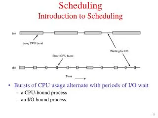
Scheduling

1. Scheduling

2. Introduction Job shop scheduling is properly defined as two interrelated tasks: 1 Job shop assignment: Assignment of machine tools to accomplish each operation on each scheduled part, and 2 Job shop sequencing: Specifying the processing order in which waiting parts are to be run on each machine tool.

3. Sequencing and Scheduling: Example Consider a job shop with machining, tapping, and inspection work centers. Today, there are two jobs waiting to be scheduled (with processing times specified in days): WC 1 WC2 WC3 Due Date Machine Tap Inspect [from today] Job 1 2 1 1 5 Job 2 3 2 1 8 Processing order for both jobs is WC1-->WC2-->WC3

4. Sequencing and Scheduling: Example There are many performance criteria that can be used to judge the �goodness� of candidate schedules. The �optimal� schedules under alternative performance criteria are likely to be different. Examples of typical scheduling performance measures Makespan - want to minimize Number of late jobs - want to minimize Maximum tardiness - want to minimize

5. Sequencing and Scheduling: Example Consider the job shop example - the jobs waiting to be processed today are both processed in the same order [and there is no choice in the assignment of jobs to machines at work centers]. Thus, there are two possible job sequence schedules: process job 1, then job 2 [1 --> 2], or process job 2, then job 1 [2 -->1].

6. Sequencing and Scheduling: Example Constructing a Gantt chart for each sequence gives:

7. Sequencing and Scheduling: Example Makespan 1 --> 2: 8 days 2 --> 1: 7 days Hence 2 --> 1 optimal Number of Late Jobs 1 --> 2: Job 1 (completed day 4 / due day 5) --> no late jobs Job 2 (completed day 8 / due day 8) 2 --> 1: Job 1 (completed day 7 / due day 5) --> Job 1 is 2 days late Job 2 (completed day 6 / due day 8) Hence 1--> 2 optimal

8. Sequencing and Scheduling: Example Maximum Tardiness 1 --> 2: no late jobs 2 --> 1: Job 1 is 2 days late Hence 1 -->2 is optimal Note: Here selection based on Late Jobs and Maximum Tardiness are the same. This is not always the case. For example, suppose we have two alternative schedules A and B Job 1 - early Job 1 - 1 day late A: Job 2 - 2 days late B: Job 2 - early Job 3 - on time Job 3 - 1 day late

9. Sequencing and Scheduling: Example To minimize number of late jobs - choose A To minimize maximum tardiness - choose B Note: Have �solved� small example problem by total enumeration of all feasible sequence schedules (here there were two) With N jobs to schedule given same processing order for each job -- have N! alternative sequence schedules With N jobs and order of processing through M operations not fixed -- have (N!)M alternative sequence schedules.

10. Sequencing and Scheduling A number of algorithms have been developed to give optimal or �very good� solutions for special cases of the sequencing problem (without requiring total enumeration). For more general forms of the sequencing problem, we will use �priority� rules to develop sequence schedules that are �good� solutions most of the time.

11. Algorithms for Sequence Scheduling The algorithms we will examine assume: Processing time estimates include set up time, and Set up time is independent of job (task) sequence

12. N Job / 1 Machine Scheduling This is the most elementary job shop scheduling problem. For this problem Makespan is independent of job processing order, i.e., let MS = Makespan associated with schedule S ti = Processing time or task i

13. Scheduling and Sequencing Definitions Time each task spends in the system may be important in terms of considerations such as in-process inventory Let Cis = Completion time for task i in schedule S = Sum of task completion times for tasks preceding task i in schedule S plus the completion time of task i

14. Scheduling and Sequencing Definitions Let Fis = Flow time for task i in schedule S = Time span from time when task i is available for processing until time when task i is completed [in schedule S] If each task is available for processing when work begins on first task, then Fis = Cis [this situation is called a static arrival pattern]

15. Scheduling and Sequencing Definitions Mean flow time for schedule If arrival pattern is static

16. N Job / 1 Machine Criterion: Minimize mean flow time [will assume static arrival pattern --> FiS = CiS] Schedule jobs so that t[1] ? t[2] ? ... ? t[N] , where t[k] = processing time for the kth task in the sequence i.e., sequence tasks (jobs) in Shortest Processing Time (SPT) order.

17. Example Given five single task jobs to be scheduled on a processor. Task ti 1 3 2 5 Scheduling in SPT order gives 3 4 5 -> 1 -> 3 -> 4 -> 2 4 4 tie, arbitrary choice 5 2

18. Lateness Can speak of lateness of task i in schedule S as: LiS = CiS - di = FiS - di [ since FiS = CiS with static arrival] (Note: negative lateness --> early) Mean lateness of schedule S = Criterion: Minimize mean lateness Schedule jobs in SPT order since = Mean flow time - constant

19. Example Given five single task jobs to be scheduled on a processor Task ti di 1 3 10 2 5 13 Scheduling in SPT order gives 3 4 9 5 -> 1 -> 3 -> 4 -> 2 4 4 13 tie, arbitrary choice 5 2 11

20. SPT Rule SPT not only minimizes mean flow time and mean lateness, it also minimizes mean waiting time and mean number of tasks waiting as in-process inventory.

21. Tardiness Define the tardiness of task i in schedule S as: TiS = max {0, CiS - di} = max {0, FiS - di} [ since FiS = CiS with static arrival] TS = max TiS for all I Criterion: Minimize maximum lateness and maximum tardiness Schedule jobs so that d[1] ? d[2] ? ... ? d[N] , where d[k] = due date for the kth task in the sequence i.e., sequence tasks (jobs) in Earliest Due Date (EDD) order

22. Example Given five single task jobs to be scheduled on a processor Task ti di 1 3 10 2 5 13 Scheduling in EDD order gives 3 4 9 3 -> 1 -> 5 -> 2 -> 4 4 4 13 tie, arbitrary choice 5 2 11

23. Hodgson�s N Job / 1 Machine Algorithm Criterion: Minimize number of late jobs 1. Sequence jobs in EDD order. 2. Identify first late job in current sequence. If late job found, go to Step 3. If no late job found, go to Step 4. 3. Examine subsequence up to and including late job. Find job in subsequence with largest processing time and reject it. Consider resulting sequence as the current sequence. Go to Step 2. 4. Current sequence, followed by rejected jobs in any order, is optimal.

24. Example Given five single task jobs to be scheduled on a processor Task ti di 1 3 10 2 5 13 Scheduling in EDD order gives 3 4 9 3 -> 1 -> 5 -> 2 -> 4 4 4 13 tie, arbitrary choice 5 2 11 we will use a helpful table format for the remaining steps

25. Example Task 3 1 5 2 4 3 1 5 4 Processing Time 4 3 2 5 4 4 3 2 4 Due Date 9 10 11 13 13 9 10 11 13 Completion Time 4 7 9 14 4 7 9 13 Optimal sequence: 3 -> 1 -> 5 -> 4 -> 2

26. M Parallel Processors Consider the job shop environment where there are M parallel processors. We schedule N single task jobs by: 1) Assigning each job (task) to one of the M machines, and then 2) We sequence jobs (tasks) at each machine

27. N Job / 1 Machine (M parallel processors) Criterion: Reduce Makespan and mean flow time 1. Sequence N jobs (tasks) in Longest Processing Time (LPT) order. 2. Schedule each task from LPT list to processor with least time already assigned. 3. After all tasks scheduled to a processor, reverse task sequence, putting tasks at each processor in SPT order.

28. Example Given six single task jobs to be scheduled on two processors Task ti di 1 5 10 2 6 12 Step 1. LPT sequence 3 4 8 2 -> 1 -> 3-> 6 -> 5 -> 4 4 2 11 tie, arbitrary choice 5 3 10 6 4 9

29. Example Step 2: Processor 1 2 --> 6 --> 4 Processing time 6 4 2 Cumulative Time 6 10 12 Processor 2 1 --> 3 --> 5 Processing Time 5 4 3 Cumulative Time 5 9 12 Step 3: Processor 1: 4 --> 6 --> 2 Processor 2: 5 --> 3 --> 1

30. N Job / 1 Machine (M parallel processors) Criterion: Reduce maximum tardiness 1. Sequence N jobs (tasks) in EDD order. 2. Schedule each task from EDD list to processor with least time already assigned.

31. Example Given six single task jobs to be scheduled on two processors Task ti di 1 5 10 2 6 12 Step 1. EDD sequence 3 4 8 3 -> 6 -> 1-> 5 -> 4 -> 2 4 2 11 tie, arbitrary choice 5 3 10 6 4 9

32. Example Step 2: Processor 1 3 --> 1 --> 2 Processing time 4 5 6 Cumulative Time 4 9 15 Processor 2 6 --> 5 --> 4 Processing Time 4 3 2 Cumulative Time 4 7 9

33. N Job / M Machine Problem Now examine more general job shop scheduling problem. Each job i has processing times ti1, ti2,...tiM indicating the amount of time required to complete processing of task 1, 2, ..., M.

34. Johnson�s N Job / 2 Machine Algorithm Criterion: Minimize Makespan Processing Order: Machine 1 then Machine 2 1. List all jobs with ti1 and ti2 entries. 2. Scan all ti1 and ti2 values to find minimum. 3. If minimum for machine 1, place corresponding job first in sequence. If minimum for machine 2, place corresponding job last in sequence. If ties for machine 1 (or 2) sequence in job subscript order. If ti1 = ti2, sequence according to machine 1. 4. Repeat steps 2 and 3 after eliminating assigned job. Continue until all jobs assigned.

35. Example Task ti1 ti2 1 5 3 2 7 8 Optimal sequence 3 9 8 2 -> 3 -> 4 -> 1 -> 5 4 4 3 5 8 2

36. Johnson�s N Job / 3 Machine Algorithm Criterion: Reduce Makespan Processing Order: Machine 1, Machine 2, then Machine 3 1. Form ti1* = ti1 + ti2, and ti2* = ti2 + ti3 2. Use Johnson�s N Job / 2 Machine Algorithm with ti1* and ti2* Johnson�s 3 Machine Algorithm generates optimal sequence if min ti1 ? max ti2 for all i for all i or min ti3 ? max ti2 for all i for all i i.e., if processing times on machine 1 or 3 dominate processing times on machine 2

37. Example Task ti1 ti2 ti3 1 7 4 9 2 9 5 7 3 3 3 6 4 6 6 8 5 5 2 10

38. Example Task ti1* ti2* 1 11 13 2 14 12 Recommended sequence 3 6 9 3 -> 5 -> 1 -> 4 -> 2 4 12 14 5 7 12 Note: recommended sequence is optimal since: min ti3 = 6 ? max ti2 = 6 for all i for all i

39. Gupta�s N job /M Machine Algorithm Processing Order: 1,2,...,M Criterion: Reduce Makespan 1. List all jobs with ti1,ti2,...,tiM in processing order. 2. Calculate the job value of each job as: JVi = K min [(ti1 + ti2), (ti2 + ti3),..., (tiM-1 +tiM)] where K = +1 if ti1 ? tiM - 1 if ti1 < tiM 3. Sequence jobs in terms of increasing job value.

40. Example Example: 3 jobs to be processed on 4 machines in the order 2,4,1,3. Job Mach. 1 Mach. 2 Mach. 3 Mach. 4 1 5 8 1 4 2 6 2 4 3 3 10 2 7 1

41. Example 1. Job ti1 ti2 ti3 ti4 1 8 4 5 1 2 2 3 6 4 3 2 1 10 7

42. Example 2. 3. Sequence 3 --> 2 -->1

43. Priority Dispatching: Extremes of Job Processing Pure job shop - job leaving a work center is equally likely to go to any other work center. Pure flow shop - all jobs follow a single route through work centers.

44. Priority Dispatching: Priority Assignments Each job is assigned a priority as it enters the job shop (or as it enters each work center) and sequencing is performed in response to the priority assignment Single set of assignments - most appropriate in a flow shop environment - generally results in �better� system performance, but hard to keep up with all jobs and insure correct processing at each work center. Assignment at each work center - most appropriate in job shop environment - generally easier to carry out.

45. Typical Priority Assignment Rules Typical priority assignment rules First come first served Last come first served Shortest processing time (SPT) Static slack: due date less time of job arrival Dynamic slack: time remaining to due date less expected (remaining) processing time

46. Evaluating Priority Assignment Rules Since most job shops run continuously, sequence optimality criteria such as total processing time and number of late jobs are not directly applicable. Generally, we judge quality of sequencing rule on basis of measures such as mean flow time and variance of flow time.

47. Evaluating Priority Assignment Rules Assessments of performance of priority rules using shop floor studies and simulations have shown that ranked in terms of mean flow time we have the following: Light 1. Shortest processing time Heavy 2. Last come first served 2. dynamic slack 3. Dynamic slack 3. Last come first served 4. First come first served 5. Static slack

48. Evaluating Priority Assignment Rules In terms of variance of flow time, rules have following ranking: 1. Dynamic slack 2. First come first served 3. Shortest processing time 4. Last come first served 5. Static slack

49. Evaluating Priority Assignment Rules In general, shortest processing time (SPT) has best overall performance characteristics - definitely smallest mean flow time, but possible for a large job to experience an extremely long flow time. One way to eliminate this problem is to use a truncated shortest processing time (TSOP) rule. With TSOP rule, jobs are SPT sequenced, but every fixed increment of time (typically day or week), large processing time jobs that have been waiting are processed.