Download

1 / 43
430 likes | 497 Views
Explore probabilistic inference in artificial intelligence, from Bayesian filtering to variable elimination and factor analysis, for efficient calculations and accurate predictions. Learn the fundamentals and applications in this advanced lecture.

E N D
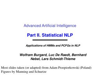
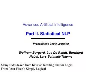
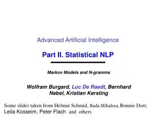
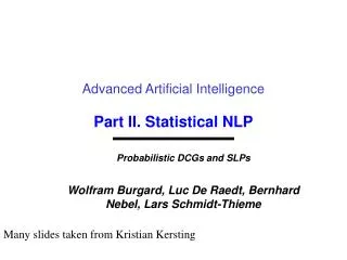
Advanced Artificial Intelligence Lecture 2C: Probabilistic Inference
Probability “Probability theory is nothing But common sense reduced to calculation.” - Pierre Laplace, 1819 The true logic for this world is the calculus of Probabilities, which takes account of the magnitude of the probability which is, or ought to be, in a reasonable man’s mind.” - James Maxwell, 1850
Probabilistic Inference • Joel Spolsky:A very senior developer who moved to Google told me that Google works and thinks at a higher level of abstraction..."Google uses Bayesian filtering the way [previous employer] uses the if statement,"he said.
Example: Alarm Network Burglary Earthquake Alarm John calls Mary calls
Probabilistic Inference • Probabilistic Inference: calculating some quantity from a joint probability distribution • Posterior probability: • In general, partition variables intoQuery (Q or X), Evidence (E), and Hidden (H or Y) variables B E A J M
Inference by Enumeration • Given unlimited time, inference in BNs is easy • Recipe: • State the unconditional probabilities you need • Enumerate all the atomic probabilities you need • Calculate sum of products • Example: B E A J M
Inference by Enumeration B E P(+b, +j, +m) = ∑e∑a P(+b, +j, +m, e, a) = ∑e∑a P(+b) P(e) P(a|+b,e) P(+j|a) P(+m|a) A J M =
Inference by Enumeration • An optimization: pull terms out of summations B E P(+b, +j, +m) = ∑e∑a P(+b, +j, +m, e, a) = ∑e∑a P(+b) P(e) P(a|+b,e) P(+j|a) P(+m|a) A J M = P(+b) ∑eP(e) ∑a P(a|+b,e) P(+j|a) P(+m|a) or = P(+b) ∑a P(+j|a) P(+m|a) ∑eP(e) P(a|+b,e)
Inference by Enumeration Problem? Not just 4 rows; approximately 1016 rows!
Causation and Correlation B E J M A A J M B E
Causation and Correlation B E M J A E J M B A
Variable Elimination • Why is inference by enumeration so slow? • You join up the whole joint distribution before you sum out (marginalize) the hidden variables( ∑e∑a P(+b) P(e) P(a|+b,e) P(+j|a) P(+m|a) ) • You end up repeating a lot of work! • Idea: interleave joining and marginalizing! • Called “Variable Elimination” • Still NP-hard, but usually much faster than inference by enumeration • Requires an algebra for combining “factors”(multi-dimensional arrays)
Variable Elimination Factors • Joint distribution: P(X,Y) • Entries P(x,y) for all x, y • Sums to 1 • Selected joint: P(x,Y) • A slice of the joint distribution • Entries P(x,y) for fixed x, all y • Sums to P(x)
Variable Elimination Factors • Family of conditionals: P(X |Y) • Multiple conditional values • Entries P(x | y) for all x, y • Sums to |Y|(e.g. 2 for Boolean Y) • Single conditional: P(Y | x) • Entries P(y | x) for fixed x, all y • Sums to 1
Variable Elimination Factors • Specified family: P(y | X) • Entries P(y | x) for fixed y, but for all x • Sums to … unknown • In general, when we write P(Y1 … YN | X1 … XM) • It is a “factor,” a multi-dimensional array • Its values are all P(y1 … yN | x1 … xM) • Any assigned X or Y is a dimension missing (selected) from the array
Example: Traffic Domain • Random Variables • R: Raining • T: Traffic • L: Late for class R T L P(L | T )
Variable Elimination Outline • Track multi-dimensional arrays called factors • Initial factors are local CPTs (one per node) • Any known values are selected • E.g. if we know , the initial factors are • VE: Alternately join factors and eliminate variables
Operation 1: Join Factors • Combining factors: • Just like a database join • Get all factors that mention the joining variable • Build a new factor over the union of the variables involved • Example: Join on R • Computation for each entry: pointwise products R R,T T
Operation 2: Eliminate • Second basic operation: marginalization • Take a factor and sum out a variable • Shrinks a factor to a smaller one • A projection operation • Example:
Example: Compute P(L) Sum out R Join R R T T R,T L L L
Example: Compute P(L) T T, L L Join T Sum out T L Early marginalization is variable elimination
Evidence • If evidence, start with factors that select that evidence • No evidence uses these initial factors: • Computing , the initial factors become: • We eliminate all vars other than query + evidence
Evidence II • Result will be a selected joint of query and evidence • E.g. for P(L | +r), we’d end up with: • To get our answer, just normalize this! • That’s it! Normalize
General Variable Elimination • Query: • Start with initial factors: • Local CPTs (but instantiated by evidence) • While there are still hidden variables (not Q or evidence): • Pick a hidden variable H • Join all factors mentioning H • Eliminate (sum out) H • Join all remaining factors and normalize
Example Choose A Σ a
Example Choose E Σ e Finish with B Normalize
Approximate Inference • Sampling / Simulating / Observing • Sampling is a hot topic in machine learning,and it is really simple • Basic idea: • Draw N samples from a sampling distribution S • Compute an approximate posterior probability • Show this converges to the true probability P • Why sample? • Learning: get samples from a distribution you don’t know • Inference: getting a sample is faster than computing the exact answer (e.g. with variable elimination) F S A
Prior Sampling Cloudy Cloudy Sprinkler Sprinkler Rain Rain WetGrass WetGrass Samples: +c, -s, +r, +w -c, +s, -r, +w …
Prior Sampling • This process generates samples with probability: …i.e. the BN’s joint probability • Let the number of samples of an event be • Then • I.e., the sampling procedure is consistent
Cloudy C Sprinkler S Rain R WetGrass W Example • We’ll get a bunch of samples from the BN: +c, -s, +r, +w +c, +s, +r, +w -c, +s, +r, -w +c, -s, +r, +w -c, -s, -r, +w • If we want to know P(W) • We have counts <+w:4, -w:1> • Normalize to get P(W) = <+w:0.8, -w:0.2> • This will get closer to the true distribution with more samples • Can estimate anything else, too • Fast: can use fewer samples if less time
Cloudy C Sprinkler S Rain R WetGrass W Rejection Sampling • Let’s say we want P(C) • No point keeping all samples around • Just tally counts of C as we go • Let’s say we want P(C| +s) • Same thing: tally C outcomes, but ignore (reject) samples which don’t have S=+s • This is called rejection sampling • It is also consistent for conditional probabilities (i.e., correct in the limit) +c, -s, +r, +w +c, +s, +r, +w -c, +s, +r, -w +c, -s, +r, +w -c, -s, -r, +w
Sampling Example 25 25 1 25 25 25 25 1 25 25 1 25 25 25 25 1 25 25 25 25 25 1 1 25 1 25 25 25 1 25 1 25 25 25 25 1 1 25 25 25 25 25 25 25 • There are 2 cups. • First: 1 penny and 1 quarter • Second: 2 quarters • Say I pick a cup uniformly at random, then pick a coin randomly from that cup. It's a quarter. What is the probability that the other coin in that cup is also a quarter? 747/1000
Likelihood Weighting • Problem with rejection sampling: • If evidence is unlikely, you reject a lot of samples • You don’t exploit your evidence as you sample • Consider P(B|+a) • Idea: fix evidence variables and sample the rest • Problem: sample distribution not consistent! • Solution: weight by probability of evidence given parents -b, -a -b, -a -b, -a -b, -a +b, +a Burglary Alarm -b +a -b, +a -b, +a -b, +a +b, +a Burglary Alarm
Likelihood Weighting • P(R|+s,+w) Cloudy Cloudy Sprinkler Sprinkler Rain Rain Samples: WetGrass WetGrass +c, +s, +r, +w 0.099 …
Cloudy C S R W Likelihood Weighting • Sampling distribution if z sampled and e fixed evidence • Now, samples have weights • Together, weighted sampling distribution is consistent
Cloudy C S Rain R W Likelihood Weighting • Likelihood weighting is good • We have taken evidence into account as we generate the sample • E.g. here, W’s value will get picked based on the evidence values of S, R • More of our samples will reflect the state of the world suggested by the evidence • Likelihood weighting doesn’t solve all our problems (P(C|+s,+r)) • Evidence influences the choice of downstream variables, but not upstream ones (C isn’t more likely to get a value matching the evidence) • We would like to consider evidence when we sample every variable
Markov Chain Monte Carlo • Idea: instead of sampling from scratch, create samples that are each like the last one. • Procedure: resample one variable at a time, conditioned on all the rest, but keep evidence fixed. E.g., for P(b|c): • Properties: Now samples are not independent (in fact they’re nearly identical), but sample averages are still consistent estimators! • What’s the point: both upstream and downstream variables condition on evidence. -b +a +c -b -a +c +b +a +c
Monty Hall Problem • Three doors, contestant chooses one. • Game show host reveals one of two remaining, knowing it does not have prize • Should contestant accept offer to switch doors? • P(+prize|¬switch) = ?P(+prize|+switch) = ?