Download
1 / 60
600 likes | 622 Views
Explore the Simulation of T in L based on Theorems 6.1, 6.2, and more. Learn about the equivalence of computability notions and simulation techniques. Dive into the proof process, including constructing programs and simulating instruction types in L.

E N D
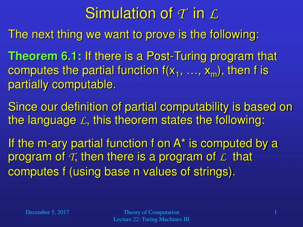
Simulation of T in L The next thing we want to prove is the following: Theorem 6.1: If there is a Post-Turing program that computes the partial function f(x1, …, xm), then f is partially computable. Since our definition of partial computability is based on the language L, this theorem states the following: If the m-ary partial function f on A* is computed by a program of T, then there is a program of L that computes f (using base n values of strings). Theory of Computation Lecture 22: Turing Machines III
Simulation of T in L Based on Theorem 6.1 and also Theorems 3.2 and 5.1, we can derive another Theorem: Theorem 6.2: Let f be an m-ary partial function on A*, where A is an alphabet of n symbols. Then the following conditions are all equivalent: 1. f is partially computable; 2. f is partially computable in Ln; 3. f is computed strictly by a Post-Turing program; 4. f is computed by a Post-Turing program. The fact that there are so many equivalent notions of computability constitutes important evidence for the correctness of Church’s Thesis. Theory of Computation Lecture 22: Turing Machines III
Simulation of T in L For the proof of Theorem 6.1, let us now consider an m-ary partial function on N. Corollary 6.3: For any n, l 1, an m-ary partial function f on N is partially computable in Ln if and only if it is also partially computable in Ll. Proof: Each of these conditions is equivalent to the function f being partially computable. Theory of Computation Lecture 22: Turing Machines III
Simulation of T in L Considering the language L1, we have: Corollary 6.4: Every partially computable function is computed strictly by some Post-Turing program that uses only the symbols s0 and s1. Proof: This follows immediately from the fact that we can simulate Ln in T, as shown before. Theory of Computation Lecture 22: Turing Machines III
Simulation of T in L Now let P be a Post-Turing program that computes f. We want to construct a program Q in the language L that computes f. Q will consist of three sections: BEGINNING MIDDLE END The MIDDLE section will simulate P in a step-by-step “interpretive” manner. The BEGINNING section will arrange the input to Q in the appropriate format for MIDDLE. The END section will extract the output. Theory of Computation Lecture 22: Turing Machines III
Simulation of T in L Let f be an m-ary partial function on A*, where A = {s1, …, sn}. The Post-Turing program P will also use the blank B and perhaps other symbols sn+1, …, sr (we are not assuming that the computation is strict). We write the symbols that P uses in the following order: s1, …, sn,sn+1, …, sr, B. The program Q will simulate P by using the numbers that strings on this alphabet represent in base r + 1 as “codes” for the corresponding strings. Theory of Computation Lecture 22: Turing Machines III
Simulation of T in L Note that we will write the blank as sr+1 instead of s0. The current tape configuration will be kept track of by Q using three numbers stored in the variables L, H, and R. H will contain the numerical value of the symbol currently being scanned by the head. L will contain a number that represents in base r + 1a string of symbols w such that the tape contents to the left of the head consists of infinitely many blanks followed by w. R will contain a number that represents in a similar manner the string of symbols to the right of the string. Theory of Computation Lecture 22: Turing Machines III
Simulation of T in L Example: Consider the following tape configuration for r = 3 (so we will use base 4): … B B B s1 s3 s2 B s1 s2 B B B … Obviously, H = 2. L = 1·4 + 3 = 7 R = 4·42 + 1·4 + 2 = 70 (remember that B = sr+1) Theory of Computation Lecture 22: Turing Machines III
Simulation of T in L We are now able to simulate all of the instruction types of T by programs of L. As usual, we will specify how to simulate each type of instruction. An instruction PRINT si is simulated in L by H i An instruction IF si GOTO L is simulated in L by IF H = i GOTO L Theory of Computation Lecture 22: Turing Machines III
Simulation of T in L An instruction RIGHT is simulated in L by L CONCATr+1(L, H) H LTENDr+1(R) R LTRUNCr+1(R) IF R 0 GOTO E R r + 1 // if R = 0, then there is a blank // (sr+1) to the right of the head Theory of Computation Lecture 22: Turing Machines III
Simulation of T in L An instruction LEFT is simulated in L by R CONCATr+1(H, R) H RTENDr+1(L) L RTRUNCr+1(L) IF L 0 GOTO E L r + 1 // if L = 0, then there is a blank // (sr+1) to the left of the head Theory of Computation Lecture 22: Turing Machines III
Simulation of T in L Now the MIDDLE section of Q can be generated by replacing each instruction in P by its simulation. When we write BEGINNING and END, we must consider the following: f is an m-ary function on {s1, …, sn}*. Thus the initial values of X1, …, Xm for Q are numbers that represent the input strings in base n. However, the computations in Q assume a base r + 1 representation of the input strings. Theory of Computation Lecture 22: Turing Machines III
Simulation of T in L Fortunately, we have Theorem 1.1 of Chapter 5, which tells us that the functions UPCHANGEn,l and DOWNCHANGEn,l are computable. Now we can develop the BEGINNING section. Its task is to calculate the initial values of L, H, and R, which represent the initial tape configuration B x1 B x2 B … B xm, where the numbers x1, …, xm are represented in base n notation. Theory of Computation Lecture 22: Turing Machines III
Simulation of T in L The BEGINNING section then looks like this: L r + 1 H r + 1 Z1 UPCHANGEn,r+1(X1) Z2 UPCHANGEn,r+1(X2) : Zm UPCHANGEn,r+1(Xm) R CONCATr+1(Z1, r + 1, Z2, r + 1, …, r + 1, Zm) Theory of Computation Lecture 22: Turing Machines III
Simulation of T in L Now let us write the END section. It is supposed to put the output of the simulated program in base n representation into variable Y. Since we are not demanding a strict computation by P , the output is the concatenation of all symbols on the tape that belong to the alphabet A = {s1, …, sn}. Therefore, our END section is written as follows: Z CONCATr+1(L, H, R) Y DOWNCHANGEn,r+1(Z) (Remember that DOWNCHANGEn,r+1 automatically removes all symbols sn+1, …, sr+1). Theory of Computation Lecture 22: Turing Machines III
Turing Machines Actually, Turing’s original model of a computer was different from the Post-Turing language. We will now look at a model that is closer to Turing’s original idea, the Turing machine. Its main difference to the Post-Turing language is that it does not read a list of instructions, but it is defined by a finite number of internal states and transitions between them. The machine’s next state is always determined by its current state and the current symbol under the head. Each transition also includes printing a symbol or moving the head one square to the left or right. Theory of Computation Lecture 22: Turing Machines III
Turing Machines The states are represented by the symbols q1, q2, q3, …, and the symbols that can appear on the tape are written as s0, s1, s2, …, where as usual s0 = B is the blank. Expressions of one of the following three forms will be referred to as quadruples: 1. qi sj sk ql 2. qi sj R ql 3. qi sj L ql They indicate that if when we are in state qi and the current symbol under the head is sj, the machine goes into state ql and 1. prints symbol sk at the current head position, 2. moves the head one square to the right, or 3. moves the head one square to the left. Theory of Computation Lecture 22: Turing Machines III
Turing Machines We now define a Turing machine to be a finite set of quadruples, no two of which begin with the same pairqi sj. This means that at any time during the computation there is no ambiguity about the next action to be performed. A Turing Machine without this requirement is called a nondeterministic Turing machine. In this course, however, we will only consider deterministic Turing machines. Theory of Computation Lecture 22: Turing Machines III
Turing Machines The alphabet of a given Turing machine M consists of all the symbols si which occur in quadruples of M except the symbol s0. A Turing machine begins its computation in state q1. A Turing machine halts if it is in state qi, scans the symbol sj, and does not have a quadruple that begins with qi sj. We use the same conventions with regard to input and output as we did for Post-Turing programs. So it should be clear what it means to say that some given Turing machine M computes a partial function f on A* for a given alphabet A. Theory of Computation Lecture 22: Turing Machines III
Turing Machines Just as for Post-Turing programs, we may speak of a Turing machine M to compute a function strictly. If M computes f, where f is a partial function on A*, we say that M computes f strictly if 1. the alphabet of M is a subset of A and 2. whenever M halts, the final configuration has the form: By qi (We indicate the current state of a Turing machine by writing the state symbol below the arrow.) Theory of Computation Lecture 22: Turing Machines III
1/R B/R B/1 B/1 1 Exit 1/R Turing Machines Example: Consider the following Turing machine with alphabet A = {1} (we will write s0 = B and s1 = 1): q1 B R q2 q2 1 R q2 q2 B 1 q3 q3 1 R q3 q3 B 1 q1 We can also represent the machine by a state transition diagram… q2 … or a table: q1 q2 q3 B 1 q1 R q2 1 q3 1 q1 q3 R q2 R q3 Theory of Computation Lecture 22: Turing Machines III
1/R q2 B/R q1 B/1 B/1 1 q3 Exit 1/R Turing Machines Now let us look at a sample computation: B111q1 B111 q2 … B111B q2 B1111 q3 B1111B q3 B11111 q1 Theory of Computation Lecture 22: Turing Machines III
Turing Machines • The previous Turing machine computes (but not strictly) the function f(x) = x + 2, where we are using unary (base 1) notation. • The steps of the computation, given by • the state of the machine, • the string of symbols on the tape, and • the square on the tape currently being scanned are called configurations. Theory of Computation Lecture 22: Turing Machines III
Another Turing Machine Example a,b/L M/L B/L q4 q3 M/R B/a a/M B/R q1 q2 Exit B a,b/R B/b b/M B/L q6 q5 a,b/L M/L Alphabet A = {a, b} Theory of Computation Lecture 22: Turing Machines III
Another Turing Machine Example a,b/L M/L B/L q4 q3 M/R B/a a/M B/R q1 q2 Exit B a,b/R B/b b/M B/L q6 q5 a,b/L M/L BbaaB q1 Theory of Computation Lecture 22: Turing Machines III
Another Turing Machine Example a,b/L M/L B/L q4 q3 M/R B/a a/M B/R q1 q2 Exit B a,b/R B/b b/M B/L q6 q5 a,b/L M/L BbaaB q2 Theory of Computation Lecture 22: Turing Machines III
Another Turing Machine Example a,b/L M/L B/L q4 q3 M/R B/a a/M B/R q1 q2 Exit B a,b/R B/b b/M B/L q6 q5 a,b/L M/L BMaaB q5 Theory of Computation Lecture 22: Turing Machines III
Another Turing Machine Example a,b/L M/L B/L q4 q3 M/R B/a a/M B/R q1 q2 Exit B a,b/R B/b b/M B/L q6 q5 a,b/L M/L BMaaB q5 Theory of Computation Lecture 22: Turing Machines III
Another Turing Machine Example a,b/L M/L B/L q4 q3 M/R B/a a/M B/R q1 q2 Exit B a,b/R B/b b/M B/L q6 q5 a,b/L M/L BBMaaB q6 Theory of Computation Lecture 22: Turing Machines III
Another Turing Machine Example a,b/L M/L B/L q4 q3 M/R B/a a/M B/R q1 q2 Exit B a,b/R B/b b/M B/L q6 q5 a,b/L M/L bBMaaB q1 Theory of Computation Lecture 22: Turing Machines III
Another Turing Machine Example a,b/L M/L B/L q4 q3 M/R B/a a/M B/R q1 q2 Exit B a,b/R B/b b/M B/L q6 q5 a,b/L M/L bBMaaB q1 Theory of Computation Lecture 22: Turing Machines III
Another Turing Machine Example a,b/L M/L B/L q4 q3 M/R B/a a/M B/R q1 q2 Exit B a,b/R B/b b/M B/L q6 q5 a,b/L M/L bBMaaB q2 Theory of Computation Lecture 22: Turing Machines III
Another Turing Machine Example a,b/L M/L B/L q4 q3 M/R B/a a/M B/R q1 q2 Exit B a,b/R B/b b/M B/L q6 q5 a,b/L M/L bBMaaB q2 Theory of Computation Lecture 22: Turing Machines III
Another Turing Machine Example a,b/L M/L B/L q4 q3 M/R B/a a/M B/R q1 q2 Exit B a,b/R B/b b/M B/L q6 q5 a,b/L M/L bBMMaB q3 Theory of Computation Lecture 22: Turing Machines III
Another Turing Machine Example a,b/L M/L B/L q4 q3 M/R B/a a/M B/R q1 q2 Exit B a,b/R B/b b/M B/L q6 q5 a,b/L M/L bBMMaB q3 Theory of Computation Lecture 22: Turing Machines III
Another Turing Machine Example a,b/L M/L B/L q4 q3 M/R B/a a/M B/R q1 q2 Exit B a,b/R B/b b/M B/L q6 q5 a,b/L M/L bBMMaB q3 Theory of Computation Lecture 22: Turing Machines III
Another Turing Machine Example a,b/L M/L B/L q4 q3 M/R B/a a/M B/R q1 q2 Exit B a,b/R B/b b/M B/L q6 q5 a,b/L M/L bBMMaB q4 Theory of Computation Lecture 22: Turing Machines III
Another Turing Machine Example a,b/L M/L B/L q4 q3 M/R B/a a/M B/R q1 q2 Exit B a,b/R B/b b/M B/L q6 q5 a,b/L M/L BbBMMaB q4 Theory of Computation Lecture 22: Turing Machines III
Another Turing Machine Example a,b/L M/L B/L q4 q3 M/R B/a a/M B/R q1 q2 Exit B a,b/R B/b b/M B/L q6 q5 a,b/L M/L abBMMaB q1 Theory of Computation Lecture 22: Turing Machines III
Another Turing Machine Example a,b/L M/L B/L q4 q3 M/R B/a a/M B/R q1 q2 Exit B a,b/R B/b b/M B/L q6 q5 a,b/L M/L abBMMaB q1 Theory of Computation Lecture 22: Turing Machines III
Another Turing Machine Example a,b/L M/L B/L q4 q3 M/R B/a a/M B/R q1 q2 Exit B a,b/R B/b b/M B/L q6 q5 a,b/L M/L abBMMaB q1 Theory of Computation Lecture 22: Turing Machines III
Another Turing Machine Example a,b/L M/L B/L q4 q3 M/R B/a a/M B/R q1 q2 Exit B a,b/R B/b b/M B/L q6 q5 a,b/L M/L abBMMaB q2 Theory of Computation Lecture 22: Turing Machines III
Another Turing Machine Example a,b/L M/L B/L q4 q3 M/R B/a a/M B/R q1 q2 Exit B a,b/R B/b b/M B/L q6 q5 a,b/L M/L abBMMaB q2 Theory of Computation Lecture 22: Turing Machines III
Another Turing Machine Example a,b/L M/L B/L q4 q3 M/R B/a a/M B/R q1 q2 Exit B a,b/R B/b b/M B/L q6 q5 a,b/L M/L abBMMaB q2 Theory of Computation Lecture 22: Turing Machines III
Another Turing Machine Example a,b/L M/L B/L q4 q3 M/R B/a a/M B/R q1 q2 Exit B a,b/R B/b b/M B/L q6 q5 a,b/L M/L abBMMMB q3 Theory of Computation Lecture 22: Turing Machines III
Another Turing Machine Example a,b/L M/L B/L q4 q3 M/R B/a a/M B/R q1 q2 Exit B a,b/R B/b b/M B/L q6 q5 a,b/L M/L abBMMMB q3 Theory of Computation Lecture 22: Turing Machines III
Another Turing Machine Example a,b/L M/L B/L q4 q3 M/R B/a a/M B/R q1 q2 Exit B a,b/R B/b b/M B/L q6 q5 a,b/L M/L abBMMMB q3 Theory of Computation Lecture 22: Turing Machines III
Another Turing Machine Example a,b/L M/L B/L q4 q3 M/R B/a a/M B/R q1 q2 Exit B a,b/R B/b b/M B/L q6 q5 a,b/L M/L abBMMMB q3 Theory of Computation Lecture 22: Turing Machines III
Another Turing Machine Example a,b/L M/L B/L q4 q3 M/R B/a a/M B/R q1 q2 Exit B a,b/R B/b b/M B/L q6 q5 a,b/L M/L abBMMMB q4 Theory of Computation Lecture 22: Turing Machines III
Another Turing Machine Example a,b/L M/L B/L q4 q3 M/R B/a a/M B/R q1 q2 Exit B a,b/R B/b b/M B/L q6 q5 a,b/L M/L abBMMMB q4 Theory of Computation Lecture 22: Turing Machines III