Download
1 / 45
460 likes | 686 Views
Figure 14.1 The UK microwave communications wideband distribution network. Figure 14.2 Splitting of a microwave frequency allocation into radio channels. Figure 14.3 Extraction (dropping) of a single radio channel in a microwave repeater.

E N D
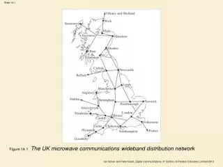
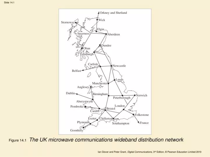
Figure 14.1 The UK microwave communications wideband distribution network
Figure 14.2 Splitting of a microwave frequency allocation into radio channels
Figure 14.3 Extraction (dropping) of a single radio channel in a microwave repeater
Figure 14.5 Schematic illustration of ducting causing overreaching
Figure 14.6 Block diagram of a typical microwave digital radio terminal
Figure 14.7 Digital DPSK regenerative repeater for a single 30 MHz radio channel
Figure 14.9 Illustration of circular paths for rays in atmosphere with vertical n-gradient (α = 0 for ray 1, α ≠ 0 for ray 2). Geometry distorted for clarity
Figure 14.10 Relative curvatures of earth’s surface and ray path in a standard atmosphere
Figure 14.12 Flat earth model (n ≈ 1 and negative radius indicates ray is concave upwards)
Figure 14.13 Characteristic ray trajectories drawn with respect to a k = 4/3 earth radius
Figure 14.14 Geometry for maximum range LOS link over a smooth, spherical, earth
Figure 14.17 Path profile for hypothetical 4 GHz LOS link designed for 0.6 Fresnel zone (FZ) clearance when k = 0.7 (O = open ground, F = forested region,W = water)
Figure 14.18 Definition of clearance, h, for knife edge diffraction
Figure 14.19 Diffraction loss over a knife edge (negative loss indicates a diffraction gain)
Figure 14.20 Specific attenuation due to gaseous constituents for transmissions through a standard atmosphere (20°C, pressure one atmosphere, water vapour content 7.5 g/m3) Source: ITU-R Handbook of Radiometeorology, 1996, with the permission of the ITU
Figure 14.21 Relationship between point and line rain rates as a function of hop length and percentage time point rain rate is exceeded Source: Hall and Barclay, 1989, reproduced with the permission of Peter Peregrinus
Figure 14.22 Specific attenuation due to rain (curves derived on the basis of spherical raindrops) Source: ITU-R Handbook of Radiometeorology, 1996, reproduced with the permission of ITU
Figure 14.23 Hydrometeor scatter causing interference between co-frequency systems
Figure 14.25 Selection of especially useful satellite orbits: (a) geostationary (GEO);(b) highly inclined highly elliptical (HIHEO); (c) polar orbit; and (d) low earth (LEO)
Figure 14.26 Coverage areas as a function of elevation angle for a satellite with global beam antenna Source: from CCIR Handbook, 1988, reproduced with the permission of ITU
Figure 14.27 Global coverage (excepting polar regions) from three geostationary satellites. (Approximately to scale, innermost circle represents 81°parallel.)
Figure 14.28 Approximate uplink (↑) and downlink (↓) allocations for region 1 (Europe, Africa, former USSR, Mongolia) fixed satellite, and broadcast satellite (BSS), services
Figure 14.30 Antenna aperture temperature, TA, in clear air (pressure one atmosphere, surface temperature 20°C, surface water vapour concentration10 g/m3) Source: ITU-R Handbook of Radiometeorology, 1996, reproduced with the permission of the ITU
Figure 14.31 Contours of EIRP with respect to EIRP on antenna boresight
Figure 14.32 Simplified block diagram of satellite transponders: (a) single conversion C-band; (b) double conversion Ku-band (redundancy not shown)
Figure 14.33 Amplitude and phase characteristic for typical satellite transponder TWT amplifier
Figure 14.35 Total ground level zenith attenuation (15°C, 1013 mb) for, A, dry atmosphere and, B, a surface water vapour content of 7.5 g/m3decaying exponentially with height Source: ITU-R Rec. P.676, 1995, reproduced with the permission of the ITU
Figure 14.37 Simplified block diagram of a traditional FDM/FM/FDMA earth station (only HPA/LNA redundancies shown)
Figure 14.38 Illustration of MCPC FDM/FM/FDMA single transponder satellite network and frequency plan for the transponder (with nine participating earth stations)
Figure 14.39 Parabolic noise power spectral density after FM demodulation
Figure 14.40 Principle of time division multiple access (TDMA)
Figure 14.41 Simplified block diagram of traditional TDM/QPSK/TDMA earth station. (Only HPA/LNA redundancies are shown.)
Figure 14.42 Typical TDMA frame structure. (DSI-AC time slot is discussed in section 14.3.7)
Figure 14.44 Satellite switched time division multiple access (SS-TDMA)