Download
1 / 29
290 likes | 482 Views
VLSI Placement. Prof. Shiyan Hu shiyan@mtu.edu Office: EERC 731. Problem formulation. Input: Blocks (standard cells and macros) B 1 , ... , B n Shapes and Pin Positions for each block B i Nets N 1 , ... , N m Output: Coordinates (x i , y i ) for block B i .

E N D
VLSI Placement Prof. Shiyan Hu shiyan@mtu.edu Office: EERC 731
Problem formulation • Input: • Blocks (standard cells and macros) B1, ... , Bn • Shapes and Pin Positions for each block Bi • Nets N1, ... , Nm • Output: • Coordinates (xi , yi ) for block Bi. • The total wire length is minimized. • Subject to area constraint or the area of the resulting block is minimized
Placement can Make A Difference Random Initial Placement Final Placement
Objective: Partitioning: Given a set of interconnected blocks, produce two sets that are of equal size, and such that the number of nets connecting the two sets is minimized.
FM Partitioning: Initial Random Placement list_of_sets = entire_chip; while(any_set_has_2_or_more_objects(list_of_sets)) { for_each_set_in(list_of_sets) { partition_it(); } /* each time through this loop the number of */ /* sets in the list doubles. */ } After Cut 1 After Cut 2
Moves are made based on object gain. Object Gain: The amount of change in cut crossings that will occur if an object is moved from its current partition into the other partition FM Partitioning: -1 2 0 - each object is assigned a gain - objects are put into a sorted gain list - the object with the highest gain is selected and moved. - the moved object is "locked" - gains of "touched" objects are recomputed - gain lists are resorted 0 -1 0 -2 0 0 -2 -1 1 -1 1
FM Partitioning: -1 2 0 0 -1 0 -2 0 0 -2 -1 1 -1 1
-1 -2 -2 0 -1 -2 -2 0 0 -2 -1 1 -1 1
-1 -2 -2 0 -1 -2 -2 0 0 -2 -1 1 1 -1
-1 -2 -2 0 -1 -2 -2 0 0 -2 -1 1 1 -1
-1 -2 -2 0 -1 -2 -2 0 -2 -2 1 -1 -1 -1
-1 -2 -2 -1 -2 0 -2 0 -2 -2 1 -1 -1 -1
-1 -2 -2 -1 -2 -2 0 0 -2 -2 1 -1 -1 -1
-1 -2 -2 1 -2 -2 0 -2 -2 -2 1 -1 -1 -1
-1 -2 -2 1 -2 -2 0 -2 -2 -2 1 -1 -1 -1
-1 -2 -2 1 -2 -2 0 -2 -2 1 -2 -1 -1 -1
-1 -2 -2 1 -2 -2 0 -1 -2 -2 -2 -3 -1 -1
-1 -2 -2 1 -2 -2 0 -1 -2 -2 -2 -3 -1 -1
-1 -2 -2 1 -2 -2 0 -1 -2 -2 -2 -3 -1 -1
-1 -2 -2 -1 -2 -2 -2 -1 -2 -2 -2 -3 -1 -1
Analytical Placement • Write down the placement problem as an analytical mathematical problem • Quadratic placement: • Sum of squared wire length is quadratic in the cell coordinates. • So the wirelength minimization problem can be formulated as a quadratic program. • It can be proved that the quadratic program is convex, hence polynomial time solvable
Example: x=100 x=200 x1 x2
Example: x=100 x=200 x1 x2 Interpretation of matrices A and B: The diagonal values A[i,i] correspond to the number of connections to xi The off diagonal values A[i,j] are -1 if object i is connected to object j, 0 otherwise The values B[i] correspond to the sum of the locations of fixed objects connected to object i
Quadratic Placement • Global optimization: solves a sequence of quadratic programming problems • Partitioning: enforces the non-overlap constraints
Partitioning • Use FM to cut.
Applying the Idea Recursively • Perform the Global Optimization again with additional constraints that the center of gravities should be in the center of regions. Center of Gravities
Process of Gordian (a) Global placement with 1 region (b) Global placement with 4 region (c) Final placements
Pros: - mathematically well behaved - efficient solution techniques Cons: - solution of Ax + B = 0 is not a legal placement, so generally some additional partitioning techniques are required. - solution of Ax + B = 0 is minimizes wirelength squared, not linear wire length. Quadratic Techniques: