
Logistic regression
Logistic regression. Analysis of proportion data. We know how many times an event occurred, and how many times did not occur. We want to know if these proportions are affected by a treatment or a factor Examples: Proportion dying Proportion responding to a treatment

Logistic regression
E N D
Presentation Transcript
Analysis of proportion data • We know how many times an event occurred, and how many times did not occur. • We want to know if these proportions are affected by a treatment or a factor • Examples: Proportion dying Proportion responding to a treatment Proportion in a sex Proportion flowering
The old fashion way: • People used to model these data using percentage mortality as the response variable • The problems with this are: • Errors are not normally distributed • The variance is not constant • The response is bounded (1-0) • We lose information of the size of the sample
However… • Some data as percentage of plant cover are better analyzed using the conventional models (normal errors and constant variance) following arcsine transformation (the response variable measured in radians)
If the response variable takes the form of percentage change is some measurement • It is usually better: • Analysis of covariance, using final weight as the response variable and initial weight as covariate, or • By specifying the response variable as a relative growth rate, measured as log(final/initial) Both of which can be analyzed with normal errors without further transformation
Rational for logistic regression • The traditional transformation of proportion data was arcsine. This transformation took care of the error distribution. There is nothing wrong with this transformation, but a simpler approach is often preferable, and is likely to produce a model easier to interpret
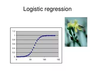
The logistic curve • The logistic curve is commonly used to describe data on proportions. • It asymptotes at 0 and 1, so that negative proportions and responses of more than 100 % cannot be predicted.
Binomial errors • If p = proportion of individuals observed to respond in a given way • The proportion of individuals that respond in alternative ways is: 1-p and we shall call this proportion q • n is the size of the sample (or number of attempts • An important point is that the variance of the binomial distribution is not constant. In fact the variance of a binomial distribution with mean np is: So that the variance changes with the mean like this:
The logistic model The logistic model for p as a function of x is given by: This model is bounded since:
The trick of linearizing the logistic model is a simple transformation See better description for the logit transformation in the class website
Hypericum cumulicola: • Small short-lived perennial herb • Narrowly endemic and endangered • Flowers are small and bisexual • Self-compatible, but requires pollinators to set seed Menges et al. (1999) Dolan et al. (1999) Boyle and Menges (2001)
Demographic data • 15 populations (various patch sizes) • >80 individuals per population each year • Data on height and number of reproductive structures • Survival between August 1994 and August 1995
Call: glm(formula = survival ~ rep_structures * height, family = binomial) Deviance Residuals: Min 1Q Median 3Q Max -2.0576 -0.9510 0.5748 0.7394 1.5518 Coefficients: Estimate Std. Error z value Pr(>|z|) (Intercept) 2.043e+00 1.888e-01 10.819 < 2e-16 *** rep_structures -9.112e-03 2.518e-03 -3.619 0.000296 *** height -2.717e-02 7.588e-03 -3.581 0.000343 *** rep_structures:height 1.219e-04 4.096e-05 2.977 0.002912 ** --- Signif. codes: 0 ‘***’ 0.001 ‘**’ 0.01 ‘*’ 0.05 ‘.’ 0.1 ‘ ’ 1 (Dispersion parameter for binomial family taken to be 1) Null deviance: 1018.68 on 878 degrees of freedom Residual deviance: 925.22 on 875 degrees of freedom AIC: 933.22 Number of Fisher Scoring iterations: 4
Calculating a given proportion • You can back-transform from logits (z) to proportions (p) by
Height - rep structures interaction 0 fruits 100 fruits survival 200 fruits 1000 fruits Height (cm)


