Download
1 / 26
260 likes | 410 Views
Opportunity Cost Algorithms for Combinatorial Auctions. by K. Akcoglu, J. Aspnes, B. DasGupta and M. Kao Presented by Yin Yang, May06. Background: Combinatorial Auction. A seller wants to sell a set O of objects.

E N D
Opportunity Cost Algorithms for Combinatorial Auctions by K. Akcoglu, J. Aspnes, B. DasGupta and M. Kao Presented by Yin Yang, May06
Background: Combinatorial Auction • A seller wants to sell a set O of objects. • A group of n competing bidders. The i-th bidder offers price pi for a set of objects Ai⊆ O. Let A = {Ai}, the set of bids. • Problem: choose a set of bids B ⊆ A, that yields maximum revenue (sum of prices paid) while being consistent (no two sets Ai and Aj in B overlap).
Background: Comb. Auction (cont.) • We construct a bid graphG = (V, E) • a node for each bid Ai, with weightpi • an edge connecting two bids if they overlap • The CA problem is transformed to computing the maximum weight independent set in G • Hopeless: this problem is not only NP-hard, but can not be approximated within ratio O(n1-ε)
Preliminaries Given G and an ordering of its nodesORD: • We say node u is a predecessor of another node v (and v a successor of u) iff. • (u, v) ∈E and • u < v according to ORD denoted as u→v • The set of predecessors (successors) are denoted as δ+(u) (δ-(u)) respectively
The OpCost Algorithm • Step 1: visit all nodes in ORD order, and compute value(u) for each node u • Step 2: visit all nodes in reverse-ORD order, and chooses node/bid u if Opportunity Cost Profitable Consistent
Theoretical Foundation (LR Lemma): Given F: a set of feasibility constraints w=w1+w2 : three weight vectors If x is an r-approximation of (F, w1) and (F, w2), then x is also an r-approximation of (F, w) Motivation: OpCost is hard to analyze, we instead analyze an equivalent algorithm LR-OpCost Idea: recursively decomposew (i.e. weight(.)) into two vectors, so that the approximation ratio can be proved by induction The LR-OpCost Algorithm
The LR-OpCost Algorithm (Cont.) • Algorithm LR-OpCost (G, w) Step 1: G2=G–{u:w(u) < 0}, return {} if G2={} Step 2: select the first node (by ORD) u in G2, and decompose w = w1+w2, where and w2 = w – w1 Step 3: B2 = LR-OpCost(G2, w2). Return B2∪{u} if it is independent, otherwise return B2.
Analysis of LR-OpCost • Theorem 2: OpCost and LR-OpCost return the same results • Proof (Sketch): Step 2 essentially computes value(.), Step 3 is the same as select(.) • Theorem 3: The approximation ratio is β(G) • See next slide • Theorem 4: The time complexity is linear to the size of G, i.e. O(|V|+|E|) • obviously
Approximation Ratios • Define: β(u) as the max size of independent set among {u} ∪ δ-(u). β = β(G) = max β(u) • Proof of approx. ratio (induction): • Base cases are trivial. • For each inductive step, assume B2 is β-approx w.r.t w2. Then B is also a β-approx w.r.t w2 , because w2(u)=0 • For w1, an upper bound of the max weight independent set is β(u)w(u)<βw(u), B gets w(u) • The bound β is tight • worst case:w(v)=1 for v with β(v)=β, and others w=1-ε
β=1 for Chordal graphs (no cycle of length >3): if G=G1∪G2, then β(G) ≤ β(G1) + β(G2); if G is node-induced sub-graph of G1, then β(G) ≤ β(G1) Given A (bid set), G and ORD, if: for each a ∈ A there is a “frontier set”Sa ⊆O of size ≤k, so that for all b that a<ORDb and a ∩ b≠{}, we have Sa ∩ b≠{}. Then β(G) ≤ k Proof: in an independent set, each successor b must intersect with Sa in a distinct element Properties of β
Constrained Combinatorial Auction In order to construct the frontier sets, we need to tweak the problem. • Observation: the objects in one bid are somehow “related” • Model: all objects for sale form an object graphH. Two objects are connected by an edge in H iff. they are “related” • Constraint: the set of objects in one bid must form a connected sub-graph of H.
Background: Tree Decomposition • A tree decomposition of H is a tree T such that each node t ∈T is associated with a set of H’s nodesVt, subject to: • ∪t ∈T Vt= V(H) • For each uv ∈E(H), ∃Vt, u∈Vt and v∈Vt • If tree node t2 lies on the path between t1 and t3, then Vt1 ∩Vt3 ⊆Vt2 • The width of a tree decomposition is max|Vt|-1, the treewidth of Htw(H) is the smallest width of any tree decompostion of H
Treewidth and β • Theorem: Given G, A, H, T and width(T) = k, we have β(G) ≤ k+1, and the ORD can be computed in linear time. • Proof: we say t1 ≤ t2 if t1 is an ancestor of t2. Extend this to a linear order of all tree nodes. For each bid a, let ta be the greatest node whose Vta intersects a. Then ORD is the order of the bids’ associated tree nodes. (next slide proves Vta is the frontier set of a)
Why Vta is the frontier set of a • Background (node removal lemma): if x, x’are not in Vt, then either (i)x and x’ are separated in H, or (ii)x and x’ are in the same connected component of T-t. • Consider bid a. Let p be the parent of ta, then a∩p={} since p>ta. Because objects in a are connected in H, (i) is eliminated. So all a’s objects are in the same subtree of T-p, which is the subtree rooted at ta. • Now consider a successor b of a, a<ORDb and a∩b≠{}. Then ∃x ∈a∩b in the subtree rooted at ta. Meanwhile, ∃x’ ∈b∩Vtb not in this subtree because tb > ta. Similarly (i) is eliminated and (ii) must hold when removing ta. The only possibility is x∈Vta.
When H is Planar Graph • Corollary: If H is planar, then ∃ORD,β(G)=O(sqrt(n)), which can be computed in O(nlogn) time. • Proof: existing algorithms can efficiently tree-decompose a planar graph achieving the width bound
Other Case Studies • Objects are intervals. β=1 • Objects are intervals partitioned into groups, each group can have only one chosen interval. (β=2) • Any β=k graph adding m such unique-selection constraints. (β=k+m) • Max-weight independent set of any subgraph of a k-dimensional grid. (β=k) • Interval selection: intervals are on a cycle. (β=2) • h-bounded height rectangle selection (β=h)
Hardness of Computing β For a general graph, β can not be efficiently computed / approximated • Theorem: If an algorithm can approximate β(G) for an n-node DAG G with ratio f(n), then it can be used to approximate the size α(H) of a max-independent set of H with ratio f(n+1) • Proof: Construct G by giving each edge an arbitrary direction and adding a new source nodes, with edges to all other nodes, we then have α(H) ≤ β(s) ≤ β(G) and β(G) ≤ α(H)
Effects of Node Ordering • Theorem (good ORD): For any G, there exists an ORD such that OpCost gets optimal answer. • Proof: Let A be any independent set in G, choose the ordering so that all nodes in A precedes all nodes not in A. Then value(u) = weight(u) ∀u∈A • Theorem (bad ORD): If all nodes in G has distinct weights, orienting G in order of decreasing weight causes OpCost to return the same results as the greedy algorithm. • Proof: by induction. value(u) = weight(u) when Greedy chooses u, otherwise value(u) < 0
A bidder whose car has broken down wants to buy either an engine, a car, or a taxi ride. Another bidder wants to buy at most three sets of car ornaments, but bid on all Yet another bidder has $100. He wants to place multiple bids worth more than that. k-of-n constraint (unweighted) Weighted budget constraint Budget Constrained CA
Unweighted Budget Constraints • Problem: bids are partitioned into groups S1, … Sr, no more than ki bids can be chosen in each group. • In OpCost, we change value(u) to • In LR-OpCost, we change w1(v) to
Analysis • Theorem: Unweighted OpCost/LR-OpCost (β+1)-approximate an optimal set of bids in linear time • Proof: the main difference from previous proof is in proving the inductive step for w1. The upper bound now becomes β(u)w(u) + ku/ku w(u) ≤ (β+1)w(u)
Overlapping Unweighted Constraints • Problem: There are r bid groups S1, … Sr each bid can appear in at most t groups. • OpCost: • LR-OpCost:
Analysis • Approximation ratio: β+t • Running time: O(|V|t+|E|) • Proof: similar to previous one
Weighted Budget Constraints • Problem: bids are partitioned into groups S1, …, Sr. For each group the total winning bids can have total value no more than bi. • Main challenge: unlike the previous cases, we can not get a good lower bound on w1-weight. • Solution: run two variations of the algorithm twice and report the better: once for heavy bids with w(v) ≥ 0.5bv and once for light bids with w(v) ≤ 0.5bv
Heavy and Light Runs • The heavy run degenerates to the unweighted case. • For the light run, we use the following w1(v)
Analysis • The heavy run obtains β+1 approximation • The light run obtains (β+2)-approx. • Overall approx. ratio is 2β+3. • Running time: linear to the size of G