Download

1 / 38
380 likes | 555 Views
8. Basic Macroeconomic Relationships. Learning objectives. In this chapter students will learn: 1. How changes in income affect consumption and saving. 2. About factors other than income that can affect consumption. 3. How changes in real interest rates affect investment.

E N D
8 Basic Macroeconomic Relationships
Learning objectives • In this chapter students will learn: 1. How changes in income affect consumption and saving. 2. About factors other than income that can affect consumption. 3. How changes in real interest rates affect investment. 4. About factors other than the real interest rate that can affect investment. 5. Why changes in investment increase or decrease real GDP by a multiple amount.
II. The Income-Consumption and Income-Saving Relationships • Disposable income is the most important determinant of consumer spending (consumption). Note that What is not spent on consumption is called saving. • Disposable Income (DI) = C + S C= consumption and S = saving Saving = DI – C • Note: • (disposable income in Kuwait = personal income since there is no income tax) • The 45-degree line: each point on the line is equidistant from the two axes. Therefore, represents all points where consumer spending is equal to disposable income.
Or each point represent a situation where; C + S = DI • Any vertical distance from the horizontal axis to the 450 line measures DI=C+S • Consumption Schedule • Reflects the direct consumption-disposable income relationship • Note: households tend to spend a larger proportion of a small DI than of a larger DI. • The saving schedule • Reflects the direct relationship between S and DI • Saving is a smaller proportion of small DI than of a large DI • Dissaving: when households consume more than their DI. They do that by liquidating their wealth (previous saving) or by borrowing (use the savings of others)
Note that “dissaving” occurs at low levels of disposable income, where consumption exceeds income and households must borrow or use up some of their wealth. • Definitions: • Average propensity to consume (APC) is the fraction or % of income consumed APC = consumption/income • Average propensity to save (APS) is the fraction or % of income saved APS = saving/income • Marginal propensity to consume (MPC) is the fraction or proportion of any change in income that is consumed MPC = change in consumption/change in income • Marginal propensity to save (MPS) is the fraction or proportion of any change in income that is saved MPS = change in saving/change in income
Note: • As DI increases; APS rises and APC falls. • APC + APS = 1 • MPC + MPS = 1 Because: • ∆DI = ∆C + ∆S • Global Perspective 8.1 shows the APCs for several nations in 2006. Note the high APCs for the U.S., Canada, and the United Kingdom.
Consumption and Saving Schedules C=97.5+0.75xDI C=-97.5+0.25xDI
CONSUMPTION AND SAVING o 45 MPC + MPS = 1 SAVING C C=97.5+0.75xDI Consumption Consumption schedule C MPC = Slope of C DISSAVING o Disposable Income MPS = Slope of S Saving schedule S C=-97.5+0.25xDI Saving SAVING o S DISSAVING Disposable Income
Break even income: • The income level at which households plan to consume their entire income, (C = DI). • At break even: • Consumption schedule cuts the 450 line. • Saving schedule cuts the horizontal axis . • Saving = zero • APC = 1 • APS = zero
(1) Level of Output And Income (GDP=DI) (4) Average Propensity to Consume (APC) (2)/(1) (5) Average Propensity to Save (APS) (3)/(1) (6) Marginal Propensity to Consume (MPC) Δ(2)/Δ(1) (7) Marginal Propensity to Save (MPS) Δ(3)/Δ(1) (2) Consump- tion (C) (3) Saving (S) (1-2) Consumption and Saving • $370 • 390 • 410 • 430 • 450 • 470 • 490 • 510 • 530 • 550 $375 390 405 420 435 450 465 480 495 510 $-5 0 5 10 15 20 25 30 35 40 1.01 1.00 .99 .98 .97 .96 .95 .94 .93 .93 -.01 .00 .01 .02 .03 .04 .05 .06 .07 .07 .75 .75 .75 .75 .75 .75 .75 .75 .75 .25 .25 .25 .25 .25 .25 .25 .25 .25
500 475 450 425 400 375 45° 50 25 0 • 390 410 430 450 470 490 510 530 550 Consumption and Saving Schedules C Saving $5 Billion Consumption Schedule Consumption (billions of dollars) Dissaving $5 Billion • 390 410 430 450 470 490 510 530 550 Disposable Income (billions of dollars) Dissaving $5 Billion Saving Schedule S Saving (billions of dollars) Saving $5 Billion
GLOBAL PERSPECTIVE Consumption and Saving Average Propensities to Consume Select Nations GDPs Average Propensities to Consume .80 .85 .90 .95 1.00 United States Canada United Kingdom Japan Germany Netherlands Italy France .963 .958 .953 .942 .896 .893 .840 .833 Source: Statistical Abstract of the United States, 2006
Nonincome determinants of consumption and saving: can cause people to spend or save more or less at various income levels, although the level of income is the basic determinant. 1. Wealth: An increase in wealth shifts the consumption schedule up and saving schedule down. Wealth Effects: when assets boast, households feel wealthy, they save less and consumer more, and vice versa. 2. Expectations: Changes in expected future prices or wealth can affect consumption spending today. 3. Real interest rates: Declining interest rates increase the incentive to borrow and consume, and reduce the incentive to save. Because many household expenditures are not interest sensitive – the light bill, groceries, etc. – the effect of interest rate changes on spending are modest. 4. Household debt:Lower debt levels shift consumption schedule up and saving schedule down. But if debt is too high, they will reduce their consumption to pay off some of their loans.
Other important considerations: • Macroeconomic models focus on real domestic output (real GDP) more than on disposable income. • Changes along schedules: Movement from one point to another on a given schedule is called a change in the amount consumed, this is due to disposable income; a shift in the schedule is called a change in consumption schedule, and is caused by non-income determinants of consumption. • Schedule shifts: Consumption and saving schedules will always shift in opposite directions unless a shift is caused by a tax change, it will shift them both in the same direction. • Taxation: Lower taxes will shift both schedules up since taxation affects both spending and saving, and vice versa for higher taxes. • Stability: Economists believe that consumption and saving schedules are generally stable unless deliberately shifted by government action.
45° Consumption and Saving Consumption and Saving Schedules C1 C0 C2 Consumption (billions of dollars) Disposable Income (billions of dollars) S2 Saving (billions of dollars) S0 S1
The Interest Rate – Investment Relationship • Investment consists of spending on new plants, capital equipment, machinery, inventories, construction, etc. • The investment decision weighs marginal benefits (r) and marginal costs (i). 1. Expected Rate of Return, r:This is marginal benefit of investment. • Expected Rate of Return= expected profit/cost of capital
If expected profit on a $1000 investment is $100. This is a 10% expected rate of return. Thus, this business would not want to pay more than a 10% interest rate on investment. • Remember that the expected rate of return is not aguaranteed rate of return. Investment carries risk. 2. Real Interest Rate, i:This is the marginal cost of investment (nominal interest rate corrected for expected inflation) Real interest rate = nominal interest rate – expected inflation
The interest rate represents either the cost of borrowed funds or the opportunity cost of investing your own funds, which is income forgone. • If real interest rate exceeds the expected rate of return, the investment should not be made, example: • If expected real rate of return r = 10% • Nominal interest rate = 15% • Inflation rate = 10% • This investment is profitable since • 10% > (i = 15%-10%) 5% • Expected return > real interest rate
Investment demand schedule, or curve, shows an inverse relationship between the interest rate and amount of investment. • As long as expected return exceeds interest rate, the investment is expected to be profitable • if rate of interest is 12%, businesses will undertake all investment opportunities that yield 12% or more. • If rate of interest is less e.g., 6%, more investment will be undertaken • If rate of interest is more, less investments will be undertaken
Cumulative Amount of Investment Having This Rate of Return or Higher (i) 16 14 12 10 8 6 4 2 0 Expected Rate of Return (r) r and i (percent) 5 10 15 20 25 30 35 40 Investment (billions of dollars) Interest Rate and Investment The Investment Demand Curve 16% 14% 12% 10% 8% 6% 4% 2% 0% $ 0 5 10 15 20 25 30 35 40 ID
Shifts in investment demand (Figure 8.6) occur when any determinant apart from the interest rate changes. 1. Greater expected returns create more investment demand; shift curve to right. The reverse causes a leftward shift. • Changes in expected returns result because of: a. Acquisition, Maintenance, and Operating Costs: Initial costs of capital, operating costs and maintenance affect the expected rate of return • When they fall, prospective investment projects increase (ID Shift to the RHS) • When they increase, prospective investment projects decrease (ID shift to the LHS)
2. Business Taxes When tax increases, expected (after tax) return decreases, shifts the investment curve to the LHS and vice versa. 3. Technological Change Technological progress (more efficient machines). Technological change often involves lower costs, which would increase expected returns and stimulates investment (shifts the investment curve to the RHS).
4. Stock of capital goods on hand Relative to output and sales, if there is abundant idle capital on hand because of weak demand or recent investment (overstock), expected return on new machines declines (would be less profitable) and investment curve shifts to the LHS and vice versa. 5. Expectations about future economic and political conditions can change the view of expected returns. • Optimistic expectations about the return, shifts the investment curve to the RHS • Pessimistic expectations shifts the investment curve to the LHS
Instability of investment Investment schedule is unstable, it shifts upward or downward quite often. Investment is the most volatile component of total spending. • Reasons for instability of investment a. Durability of capital Within limits, purchases of capital goods are discretionary and therefore, can be postponed. Optimism about future may prompt firms to replace older capital. Pessimism about the future lead to small investment as firms repair old capital and postpone new.
b. Irregularity of Innovation Technological progress is a major determinant of investment. But major innovations occur quite irregularly. When they happen, they induce vast investments. e.g., the new information technology c. Variability of profits: Profits are highly variable. This contributes to the volatile incentive to invest. Also profits are a major source of investment finance (internal source), if they are variable, investment will be instable.
d. Variability of expectations • Expectations are influenced by: • Current profit levels, • Changes in exchange rates, • Outlook for international peace, • Changes in government policies • Stock market prices…etc
GLOBAL PERSPECTIVE Interest Rate and Investment Gross Investment Expenditures as a Percent of GDP, Select Nations Percent of GDP, 2004 0 10 20 30 South Korea Japan Mexico Canada France United States Germany United Kingdom Sweden Source: World Bank
Interest Rate and Investment The Volatility of Investment Gross Investment Percentage Change GDP 1971 1975 1979 1983 1987 1991 1995 1999 2003 Year
IV. The Multiplier Effect A. Changes in spending ripple through the economy to generate event larger changes in real GDP. This is called the multiplier effect. • Multiplier= change in real GDP / initial change in spending. Alternatively, it can be rearranged to read: • Change in real GDP= initial change in spending x multiplier. • Three points to remember about the multiplier: a. The initial change in spending is usually associated with investment because it is so volatile, but changes in consumption (unrelated to income), net exports, and government purchases also are subject to the multiplier effect. b. The initial change refers to an upshift or downshift in the aggregate expenditures schedule due to a change in one of its components, like investment. c. The multiplier works in both directions (up or down).
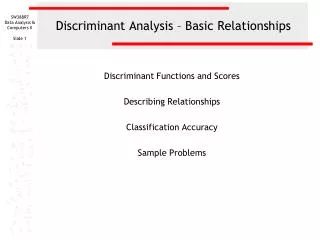
The multiplier is based on two facts. 1. The economy has continuous flows of expenditures and income—a ripple effect—in which income received by X comes from money spent by Y. Y’s income, in turn, came from money spent by Z, and so forth. 2. Any change in income will cause both consumption and saving to vary in the same direction as the initial change in income, and by a fraction of that change. Note that: a. The fraction of the change in income that is spent is called the marginal propensity to consume (MPC). b. The fraction of the change in income that is saved is called the marginal propensity to save (MPS). c. This is illustrated in Table 8.3, and Figure 8.8 that is derived from the Table. d. The size of the MPC and the multiplier are directly related; the size of the MPS and the multiplier are inversely related. See Figure 8.9 for an illustration of this point. In equation form Multiplier = 1 / MPS or 1 / (1-MPC).
The significance of the multiplier is that a small change in investment plans or consumption-saving plans can trigger a much larger change in the equilibrium level of GDP. • The simple multiplier given above can be generalized to include other “leakages” from the spending flow besides savings. For example, the actual multiplier is derived by including taxes and imports as well as savings in the equation. In other words, the denominator is the fraction of a change in income not spent on domestic output. (Key Question 9)
The Multiplier Effect Tabular and Graphical Views (2) Change in Consumption (MPC = .75) (3) Change in Saving (MPs = .25) (1) Change in Income Increase in Investment of $5 Second Round Third Round Fourth Round Fifth Round All other rounds Total $ 5.00 3.75 2.81 2.11 1.58 4.75 $ 20.00 $ 3.75 2.81 2.11 1.58 1.19 3.56 $ 15.00 $ 1.25 .94 .70 .53 .39 1.19 $ 5.00 $20.00 $4.75 15.25 $1.58 13.67 $2.11 11.56 $2.81 8.75 ΔI= $5 billion $3.75 5.00 $5.00 1 2 3 4 5 All Rounds of Spending
The Multiplier Effect The MPC and the Multiplier MPC Multiplier .9 10 .8 5 .75 4 .67 3 .5 2
Squaring the Economic Circle Last Word • Humorist Art Buchwald and the Multiplier • One Person Can’t Buy a Product • Others Subsequently Impacted and Cannot Buy Other Items • Multiple Effects Impact Psyche • Ultimately Causes Multiple Step Impact Upon the Economy as a Whole
45° (degree) line consumption schedule saving schedule break-even income average propensity to consume (APC) average propensity to save (APS) marginal propensity to consume (MPC) marginal propensity to save (MPS) wealth effect expected rate of return investment demand curve multiplier Key Terms
Next Chapter Preview… The Aggregate Expenditures Model Chapter 9!